Logistic regression classifier tutorial.
로지스틱 회귀 분류기
목차
8.특징 벡터(feature vector) 및 타겟 변수 선언
12.모델훈련
13.결과 예측
14.정확도 확인
16.류 성능 평가 지표
17.임계값 조정
18.ROC - AUC(Receiver Operating Characteristic Curve)
20.GridSearch CV를 사용한 하이퍼파라미터 최적화
21.결과 및 결론
1.로지스틱 회귀 소개
다양한 분류 문제를 해결하는 데 사용되는 알고리즘 중 하나인 로지스틱 회귀는 이산 집합의 클래스로 관측치를 예측하는 데 사용되는 지도 학습 분류 알고리즘입니다. 실제로, 관측치를 서로 다른 범주로 분류하는 데 사용됩니다.
2. 로스스틱 회귀의 직관적인 이해
통계학에서 로지스틱 회귀 모델은 주로 분류를 위해 사용됩니다. 즉, 주어진 관측치 집합에 대해 로지스틱 회귀 알고리즘을 사용하여 해당 관측치를 두 개 이상의 이산적인 클래스로 분류할 수 있습니다. 이때 대상 변수는 이산적인 특성을 가지게 됩니다.
로지스틱 회귀 알고리즘은 다음과 같습니다.
선형 방정식 구현
로지스틱 회귀 알고리즘은 독립 변수 또는 설명 변수와 함께 선형 방정식을 구현하여 반응 값을 예측하는 방식으로 작동합니다. 예를 들어, 우리는 공부한 시간과 시험 통과 확률에서 공부한 시간은 설명 변수이며 x1으로 표시됩니다. 시험 통과 확률은 반응 또는 대상 변수이며 z로 표시됩니다.
하나의 설명 변수(x1) 와 하나의 반응 변수(z) 가 있는 경우, 선형 방정식은 다음과 같은 수학적 방정식으로 주어집니다. (계수 β0과 β1은 모델의 매개 변수)
z = β0 + β1x1
여러 개의 설명 변수가 있는 경우에서 예측된 반응 값은 아래의 방정식으로 주어지며, z로 표시됩니다. (계수 β0, β1, β2 및 βn은 모델의 매개 변수)
z = β0 + β1x1+ β2x2+……..+ βnxn
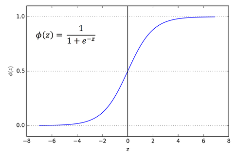
시그모이드 함수
이러한 예측된 반응 값 z는 0과 1 사이의 확률 값으로 변환됩니다.다. 다시 말해 sigmoid 함수를 사용하여 예측된 값들을 임의의 실수 값을 0과 1 사이의 확률 값으로 매핑합니다. (여기서 매핑이란 하나의 값을 다른 값으로 대응시키는 것을 말합니다.)
sigmoid 함수는 로지스틱 함수의 특수한 경우입니다. 이는 S 모양 곡선을 가지며, sigmoid 곡선이라고도 합니다.
아래의 그래프가 sigmoid 함수의 그래프의 예시 입니다.
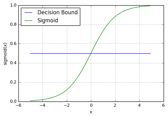
결정 경계
sigmoid 함수가 반환하는 0과 1 사이의 확률 값은 “0” 또는 “1”인 이산 클래스에 매핑됩니다. 이 확률 값을 이산 클래스 (합격 / 불합격, 예 / 아니오, 참 / 거짓)에 매핑하려면 임계값을 선택해야 합니다. 이 임계값을 결정 경계(Decision boundary)라고 합니다. 이 임계값을 기준으로, 임계값 이상인 경우 확률 값을 클래스 1로 매핑하고, 임계값 이하인 경우 확률 값을 클래스 0으로 매핑합니다.
수학적으로 다음과 같이 표현할 수 있습니다.
p ≥ 0.5 => class = 1
p < 0.5 => class = 0
일반적으로, 결정 경계는 0.5로 설정됩니다. 따라서, 아래 그림처럼 확률 값이 0.8 (> 0.5)이면 이 관측치를 클래스 1로 매핑하고 확률 값이 0.2 (< 0.5)이면 이 관측치를 클래스 0으로 매핑합니다.
예측하기
시그모이드 함수와 결정 경계를 활용하여 예측 함수를 작성할 수 있습니다. 로지스틱 회귀에서의 예측 함수는 관측값이 양성, Yes 또는 True일 확률을 반환합니다. 이를 class 1이라고 하며 P(class=1)로 표시합니다. 확률이 1에 가까워질수록 관측값이 class 1에 속할 가능성이 높아지며, 그렇지 않으면 class 0에 속할 가능성이 높아집니다.
3.로지스틱 회귀의 가정
로지스틱 회귀 모델은 다음과 같은 가정이 필요합니다.
-
로지스틱 회귀 모델은 종속 변수가 이진(binary), 다항(multinomial) 또는 순서형(ordinal)이어야 함
-
각 관측치는 반복측정에서 나온 것이 아닌, 서로 독립적이어야 함
-
독립 변수들 사이에는 다중공선성(multicollinearity)이 적거나 없어야 합니다. (다중공선성-독립 변수들 간에 높은 상관관계가 있어서 모델의 예측 능력이 저하되는 현상)
-
로지스틱 회귀 모델은 독립 변수와 로그 오즈의 선형성(linearity)을 가정
-
로지스틱 회귀 모델의 성공은 샘플 크기에 따라 달라짐. 일반적으로 높은 정확도를 달성하려면 큰 샘플 크기가 필요
4.로지스틱 회귀 유형
로지스틱 회귀 모델은 타겟 변수 범주에 따라 세 가지 그룹으로 분류될 수 있습니다.
1. 이항 로지스틱 회귀
이항 로지스틱 회귀에서 타겟 변수는 yes 또는 no, good 또는 bad, true 또는 false, 스팸 또는 스팸이 아님, 합격 또는 불합격과 같은 두 개의 범주를 가지고 있습니다.
2. 다항 로지스틱 회귀
다항 로지스틱 회귀에서 타겟 변수는 과일의 종류 - 사과, 망고, 오렌지, 바나나와 같은 세 개 이상의 범주가 있으며 특정한 순서가 없습니다. 따라서 세 개 이상의 명목적 범주가 있습니다.
3. 순서 로지스틱 회귀
순서 로지스틱 회귀에서 타겟 변수는 학생의 성적이 poor, average, good, excellent와 같은 세 개 이상의 범주 간 순서가 있는 순서 범주를 가지고 있습니다.
5. 라이브러리 가져오기
import sys
!{sys.executable} -m pip install pandas numpy
!pip install matplotlib
!pip install seaborn
Requirement already satisfied: pandas in c:\users\보일우\appdata\local\programs\python\python310\lib\site-packages (2.0.0)
Requirement already satisfied: numpy in c:\users\보일우\appdata\local\programs\python\python310\lib\site-packages (1.24.2)
Requirement already satisfied: tzdata>=2022.1 in c:\users\보일우\appdata\local\programs\python\python310\lib\site-packages (from pandas) (2023.3)
Requirement already satisfied: pytz>=2020.1 in c:\users\보일우\appdata\local\programs\python\python310\lib\site-packages (from pandas) (2023.3)
Requirement already satisfied: python-dateutil>=2.8.2 in c:\users\보일우\appdata\local\programs\python\python310\lib\site-packages (from pandas) (2.8.2)
Requirement already satisfied: six>=1.5 in c:\users\보일우\appdata\local\programs\python\python310\lib\site-packages (from python-dateutil>=2.8.2->pandas) (1.16.0)


[notice] A new release of pip available: 22.2.2 -> 23.1
[notice] To update, run: python.exe -m pip install --upgrade pip


Requirement already satisfied: matplotlib in c:\users\보일우\appdata\local\programs\python\python310\lib\site-packages (3.7.1)
Requirement already satisfied: fonttools>=4.22.0 in c:\users\보일우\appdata\local\programs\python\python310\lib\site-packages (from matplotlib) (4.39.3)
Requirement already satisfied: pyparsing>=2.3.1 in c:\users\보일우\appdata\local\programs\python\python310\lib\site-packages (from matplotlib) (3.0.9)
Requirement already satisfied: python-dateutil>=2.7 in c:\users\보일우\appdata\local\programs\python\python310\lib\site-packages (from matplotlib) (2.8.2)
Requirement already satisfied: kiwisolver>=1.0.1 in c:\users\보일우\appdata\local\programs\python\python310\lib\site-packages (from matplotlib) (1.4.4)
Requirement already satisfied: contourpy>=1.0.1 in c:\users\보일우\appdata\local\programs\python\python310\lib\site-packages (from matplotlib) (1.0.7)
Requirement already satisfied: cycler>=0.10 in c:\users\보일우\appdata\local\programs\python\python310\lib\site-packages (from matplotlib) (0.11.0)
Requirement already satisfied: packaging>=20.0 in c:\users\보일우\appdata\local\programs\python\python310\lib\site-packages (from matplotlib) (23.0)
Requirement already satisfied: numpy>=1.20 in c:\users\보일우\appdata\local\programs\python\python310\lib\site-packages (from matplotlib) (1.24.2)
Requirement already satisfied: pillow>=6.2.0 in c:\users\보일우\appdata\local\programs\python\python310\lib\site-packages (from matplotlib) (9.5.0)
Requirement already satisfied: six>=1.5 in c:\users\보일우\appdata\local\programs\python\python310\lib\site-packages (from python-dateutil>=2.7->matplotlib) (1.16.0)


[notice] A new release of pip available: 22.2.2 -> 23.1
[notice] To update, run: python.exe -m pip install --upgrade pip


Requirement already satisfied: seaborn in c:\users\보일우\appdata\local\programs\python\python310\lib\site-packages (0.12.2)
Requirement already satisfied: numpy!=1.24.0,>=1.17 in c:\users\보일우\appdata\local\programs\python\python310\lib\site-packages (from seaborn) (1.24.2)
Requirement already satisfied: matplotlib!=3.6.1,>=3.1 in c:\users\보일우\appdata\local\programs\python\python310\lib\site-packages (from seaborn) (3.7.1)
Requirement already satisfied: pandas>=0.25 in c:\users\보일우\appdata\local\programs\python\python310\lib\site-packages (from seaborn) (2.0.0)
Requirement already satisfied: python-dateutil>=2.7 in c:\users\보일우\appdata\local\programs\python\python310\lib\site-packages (from matplotlib!=3.6.1,>=3.1->seaborn) (2.8.2)
Requirement already satisfied: pyparsing>=2.3.1 in c:\users\보일우\appdata\local\programs\python\python310\lib\site-packages (from matplotlib!=3.6.1,>=3.1->seaborn) (3.0.9)
Requirement already satisfied: kiwisolver>=1.0.1 in c:\users\보일우\appdata\local\programs\python\python310\lib\site-packages (from matplotlib!=3.6.1,>=3.1->seaborn) (1.4.4)
Requirement already satisfied: fonttools>=4.22.0 in c:\users\보일우\appdata\local\programs\python\python310\lib\site-packages (from matplotlib!=3.6.1,>=3.1->seaborn) (4.39.3)
Requirement already satisfied: pillow>=6.2.0 in c:\users\보일우\appdata\local\programs\python\python310\lib\site-packages (from matplotlib!=3.6.1,>=3.1->seaborn) (9.5.0)
Requirement already satisfied: cycler>=0.10 in c:\users\보일우\appdata\local\programs\python\python310\lib\site-packages (from matplotlib!=3.6.1,>=3.1->seaborn) (0.11.0)
Requirement already satisfied: packaging>=20.0 in c:\users\보일우\appdata\local\programs\python\python310\lib\site-packages (from matplotlib!=3.6.1,>=3.1->seaborn) (23.0)
Requirement already satisfied: contourpy>=1.0.1 in c:\users\보일우\appdata\local\programs\python\python310\lib\site-packages (from matplotlib!=3.6.1,>=3.1->seaborn) (1.0.7)
Requirement already satisfied: pytz>=2020.1 in c:\users\보일우\appdata\local\programs\python\python310\lib\site-packages (from pandas>=0.25->seaborn) (2023.3)
Requirement already satisfied: tzdata>=2022.1 in c:\users\보일우\appdata\local\programs\python\python310\lib\site-packages (from pandas>=0.25->seaborn) (2023.3)
Requirement already satisfied: six>=1.5 in c:\users\보일우\appdata\local\programs\python\python310\lib\site-packages (from python-dateutil>=2.7->matplotlib!=3.6.1,>=3.1->seaborn) (1.16.0)


[notice] A new release of pip available: 22.2.2 -> 23.1
[notice] To update, run: python.exe -m pip install --upgrade pip
# This Python 3 environment comes with many helpful analytics libraries installed
# It is defined by the kaggle/python docker image: https://github.com/kaggle/docker-python
# For example, here's several helpful packages to load in

import numpy as np # linear algebra
import pandas as pd # data processing, CSV file I/O (e.g. pd.read_csv)
import matplotlib.pyplot as plt # data visualization
import seaborn as sns # statistical data visualization
%matplotlib inline

# Input data files are available in the "../input/" directory.
# For example, running this (by clicking run or pressing Shift+Enter) will list all files under the input directory

import os
for dirname, _, filenames in os.walk('/kaggle/input'):
    for filename in filenames:
        print(os.path.join(dirname, filename))

# Any results you write to the current directory are saved as output.
import warnings

warnings.filterwarnings('ignore')
6. 데이터셋 불러오기
data = 'weatherAUS.csv'

df = pd.read_csv(data)
7. 탐색적 데이터 분석
데이터 세트에 142193개의 인스턴스와 24개의 변수가 있습니다.
# view dimensions of dataset

df.shape
(145460, 23)
# preview the dataset

df.head()
| Date | Location | MinTemp | MaxTemp | Rainfall | Evaporation | Sunshine | WindGustDir | WindGustSpeed | WindDir9am | ... | Humidity9am | Humidity3pm | Pressure9am | Pressure3pm | Cloud9am | Cloud3pm | Temp9am | Temp3pm | RainToday | RainTomorrow | |
|---|---|---|---|---|---|---|---|---|---|---|---|---|---|---|---|---|---|---|---|---|---|
| 0 | 2008-12-01 | Albury | 13.4 | 22.9 | 0.6 | NaN | NaN | W | 44.0 | W | ... | 71.0 | 22.0 | 1007.7 | 1007.1 | 8.0 | NaN | 16.9 | 21.8 | No | No |
| 1 | 2008-12-02 | Albury | 7.4 | 25.1 | 0.0 | NaN | NaN | WNW | 44.0 | NNW | ... | 44.0 | 25.0 | 1010.6 | 1007.8 | NaN | NaN | 17.2 | 24.3 | No | No |
| 2 | 2008-12-03 | Albury | 12.9 | 25.7 | 0.0 | NaN | NaN | WSW | 46.0 | W | ... | 38.0 | 30.0 | 1007.6 | 1008.7 | NaN | 2.0 | 21.0 | 23.2 | No | No |
| 3 | 2008-12-04 | Albury | 9.2 | 28.0 | 0.0 | NaN | NaN | NE | 24.0 | SE | ... | 45.0 | 16.0 | 1017.6 | 1012.8 | NaN | NaN | 18.1 | 26.5 | No | No |
| 4 | 2008-12-05 | Albury | 17.5 | 32.3 | 1.0 | NaN | NaN | W | 41.0 | ENE | ... | 82.0 | 33.0 | 1010.8 | 1006.0 | 7.0 | 8.0 | 17.8 | 29.7 | No | No |
5 rows × 23 columns
col_names = df.columns

col_names
Index(['Date', 'Location', 'MinTemp', 'MaxTemp', 'Rainfall', 'Evaporation',
       'Sunshine', 'WindGustDir', 'WindGustSpeed', 'WindDir9am', 'WindDir3pm',
       'WindSpeed9am', 'WindSpeed3pm', 'Humidity9am', 'Humidity3pm',
       'Pressure9am', 'Pressure3pm', 'Cloud9am', 'Cloud3pm', 'Temp9am',
       'Temp3pm', 'RainToday', 'RainTomorrow'],
      dtype='object')
df.info()
<class 'pandas.core.frame.DataFrame'>
RangeIndex: 145460 entries, 0 to 145459
Data columns (total 23 columns):
 #   Column         Non-Null Count   Dtype
---  ------         --------------   -----
 0   Date           145460 non-null  object
 1   Location       145460 non-null  object
 2   MinTemp        143975 non-null  float64
 3   MaxTemp        144199 non-null  float64
 4   Rainfall       142199 non-null  float64
 5   Evaporation    82670 non-null   float64
 6   Sunshine       75625 non-null   float64
 7   WindGustDir    135134 non-null  object
 8   WindGustSpeed  135197 non-null  float64
 9   WindDir9am     134894 non-null  object
 10  WindDir3pm     141232 non-null  object
 11  WindSpeed9am   143693 non-null  float64
 12  WindSpeed3pm   142398 non-null  float64
 13  Humidity9am    142806 non-null  float64
 14  Humidity3pm    140953 non-null  float64
 15  Pressure9am    130395 non-null  float64
 16  Pressure3pm    130432 non-null  float64
 17  Cloud9am       89572 non-null   float64
 18  Cloud3pm       86102 non-null   float64
 19  Temp9am        143693 non-null  float64
 20  Temp3pm        141851 non-null  float64
 21  RainToday      142199 non-null  object
 22  RainTomorrow   142193 non-null  object
dtypes: float64(16), object(7)
memory usage: 25.5+ MB
변수의 종류
이 섹션에서는 데이터셋을 데이터 타입이 object인 범주형 변수와 데이터 타입이 float64인 수치형 변수로 구분합니다. 데이터셋에는 범주형 변수와 수치형 변수가 혼합되어 있습니다.
우선, 범주형 변수를 보면
# find categorical variables

categorical = [var for var in df.columns if df[var].dtype=='O']

print('There are {} categorical variables\n'.format(len(categorical)))

print('The categorical variables are :', categorical)
There are 7 categorical variables

The categorical variables are : ['Date', 'Location', 'WindGustDir', 'WindDir9am', 'WindDir3pm', 'RainToday', 'RainTomorrow']
# view the categorical variables

df[categorical].head()
| Date | Location | WindGustDir | WindDir9am | WindDir3pm | RainToday | RainTomorrow | |
|---|---|---|---|---|---|---|---|
| 0 | 2008-12-01 | Albury | W | W | WNW | No | No |
| 1 | 2008-12-02 | Albury | WNW | NNW | WSW | No | No |
| 2 | 2008-12-03 | Albury | WSW | W | WSW | No | No |
| 3 | 2008-12-04 | Albury | NE | SE | E | No | No |
| 4 | 2008-12-05 | Albury | W | ENE | NW | No | No |
범주형 변수 요약
- 데이터셋에는 Date 열로 표시되는 날짜 변수가 있음.
- Location, WindGustDir, WindDir9am, WindDir3pm, WindDir9am, WindDir3pm, RainToday 및 RainTomorrow과 같이 6개의 범주형 변수가 있음
- RainToday와 RainTomorrow은 이진 범주형 변수
- RainTomorrow은 타겟 변수
범주형 변수 내에서 문제 탐색
범주형 변수의 결측값
# check missing values in categorical variables

df[categorical].isnull().sum()
Date                0
Location            0
WindGustDir     10326
WindDir9am      10566
WindDir3pm       4228
RainToday        3261
RainTomorrow     3267
dtype: int64
# print categorical variables containing missing values

cat1 = [var for var in categorical if df[var].isnull().sum()!=0]

print(df[cat1].isnull().sum())
WindGustDir     10326
WindDir9am      10566
WindDir3pm       4228
RainToday        3261
RainTomorrow     3267
dtype: int64
우리는 여기서 데이터셋에 WindGustDir, WindDir9am, WindDir3pm 및 RainToday의 4가지 범주형 변수에만 결측값이 있음을 알 수 있습니다.
범주형 변수의 빈도수
# view frequency of categorical variables

for var in categorical:

    print(df[var].value_counts())
Date
2013-11-12    49
2014-09-01    49
2014-08-23    49
2014-08-24    49
2014-08-25    49
              ..
2007-11-29     1
2007-11-28     1
2007-11-27     1
2007-11-26     1
2008-01-31     1
Name: count, Length: 3436, dtype: int64
Location
Canberra            3436
Sydney              3344
Darwin              3193
Melbourne           3193
Brisbane            3193
Adelaide            3193
Perth               3193
Hobart              3193
Albany              3040
MountGambier        3040
Ballarat            3040
Townsville          3040
GoldCoast           3040
Cairns              3040
Launceston          3040
AliceSprings        3040
Bendigo             3040
Albury              3040
MountGinini         3040
Wollongong          3040
Newcastle           3039
Tuggeranong         3039
Penrith             3039
Woomera             3009
Nuriootpa           3009
Cobar               3009
CoffsHarbour        3009
Moree               3009
Sale                3009
PerthAirport        3009
PearceRAAF          3009
Witchcliffe         3009
BadgerysCreek       3009
Mildura             3009
NorfolkIsland       3009
MelbourneAirport    3009
Richmond            3009
SydneyAirport       3009
WaggaWagga          3009
Williamtown         3009
Dartmoor            3009
Watsonia            3009
Portland            3009
Walpole             3006
NorahHead           3004
SalmonGums          3001
Katherine           1578
Nhil                1578
Uluru               1578
Name: count, dtype: int64
WindGustDir
W      9915
SE     9418
N      9313
SSE    9216
E      9181
S      9168
WSW    9069
SW     8967
SSW    8736
WNW    8252
NW     8122
ENE    8104
ESE    7372
NE     7133
NNW    6620
NNE    6548
Name: count, dtype: int64
WindDir9am
N      11758
SE      9287
E       9176
SSE     9112
NW      8749
S       8659
W       8459
SW      8423
NNE     8129
NNW     7980
ENE     7836
NE      7671
ESE     7630
SSW     7587
WNW     7414
WSW     7024
Name: count, dtype: int64
WindDir3pm
SE     10838
W      10110
S       9926
WSW     9518
SSE     9399
SW      9354
N       8890
WNW     8874
NW      8610
ESE     8505
E       8472
NE      8263
SSW     8156
NNW     7870
ENE     7857
NNE     6590
Name: count, dtype: int64
RainToday
No     110319
Yes     31880
Name: count, dtype: int64
RainTomorrow
No     110316
Yes     31877
Name: count, dtype: int64
# view frequency distribution of categorical variables

for var in categorical:

    print(df[var].value_counts()/float(len(df)))
Date
2013-11-12    0.000337
2014-09-01    0.000337
2014-08-23    0.000337
2014-08-24    0.000337
2014-08-25    0.000337
                ...
2007-11-29    0.000007
2007-11-28    0.000007
2007-11-27    0.000007
2007-11-26    0.000007
2008-01-31    0.000007
Name: count, Length: 3436, dtype: float64
Location
Canberra            0.023622
Sydney              0.022989
Darwin              0.021951
Melbourne           0.021951
Brisbane            0.021951
Adelaide            0.021951
Perth               0.021951
Hobart              0.021951
Albany              0.020899
MountGambier        0.020899
Ballarat            0.020899
Townsville          0.020899
GoldCoast           0.020899
Cairns              0.020899
Launceston          0.020899
AliceSprings        0.020899
Bendigo             0.020899
Albury              0.020899
MountGinini         0.020899
Wollongong          0.020899
Newcastle           0.020892
Tuggeranong         0.020892
Penrith             0.020892
Woomera             0.020686
Nuriootpa           0.020686
Cobar               0.020686
CoffsHarbour        0.020686
Moree               0.020686
Sale                0.020686
PerthAirport        0.020686
PearceRAAF          0.020686
Witchcliffe         0.020686
BadgerysCreek       0.020686
Mildura             0.020686
NorfolkIsland       0.020686
MelbourneAirport    0.020686
Richmond            0.020686
SydneyAirport       0.020686
WaggaWagga          0.020686
Williamtown         0.020686
Dartmoor            0.020686
Watsonia            0.020686
Portland            0.020686
Walpole             0.020665
NorahHead           0.020652
SalmonGums          0.020631
Katherine           0.010848
Nhil                0.010848
Uluru               0.010848
Name: count, dtype: float64
WindGustDir
W      0.068163
SE     0.064746
N      0.064024
SSE    0.063358
E      0.063117
S      0.063028
WSW    0.062347
SW     0.061646
SSW    0.060058
WNW    0.056730
NW     0.055837
ENE    0.055713
ESE    0.050681
NE     0.049038
NNW    0.045511
NNE    0.045016
Name: count, dtype: float64
WindDir9am
N      0.080833
SE     0.063846
E      0.063083
SSE    0.062643
NW     0.060147
S      0.059528
W      0.058153
SW     0.057906
NNE    0.055885
NNW    0.054860
ENE    0.053870
NE     0.052736
ESE    0.052454
SSW    0.052159
WNW    0.050969
WSW    0.048288
Name: count, dtype: float64
WindDir3pm
SE     0.074508
W      0.069504
S      0.068239
WSW    0.065434
SSE    0.064616
SW     0.064306
N      0.061116
WNW    0.061006
NW     0.059192
ESE    0.058470
E      0.058243
NE     0.056806
SSW    0.056070
NNW    0.054104
ENE    0.054015
NNE    0.045305
Name: count, dtype: float64
RainToday
No     0.758415
Yes    0.219167
Name: count, dtype: float64
RainTomorrow
No     0.758394
Yes    0.219146
Name: count, dtype: float64
레이블 수: cardinality
카테고리 변수 내의 레이블 수를 카디널리티(cardinality) 라고 합니다. 변수 내 레이블 수가 많을수록 고 카디널리티(high card inality) 라고 합니다. 고 카디널리티는 머신러닝 모델에서 심각한 문제를 일으킬 수 있으므로, 고 카디널리티를 확인해야 합니다.
# check for cardinality in categorical variables

for var in categorical:

    print(var, ' contains ', len(df[var].unique()), ' labels')
Date  contains  3436  labels
Location  contains  49  labels
WindGustDir  contains  17  labels
WindDir9am  contains  17  labels
WindDir3pm  contains  17  labels
RainToday  contains  3  labels
RainTomorrow  contains  3  labels
날짜 변수(Date)에서 많은 변수를 포함하므로 해당 변수를 전처리해야합니다.
날짜 변수의 Feature Engineering
df['Date'].dtypes
dtype('O')
현재 object로 코딩된 날짜를 datetime 형식으로 파싱합니다.
# parse the dates, currently coded as strings, into datetime format

df['Date'] = pd.to_datetime(df['Date'])
# extract year from date

df['Year'] = df['Date'].dt.year

df['Year'].head()
0    2008
1    2008
2    2008
3    2008
4    2008
Name: Year, dtype: int32
# extract month from date

df['Month'] = df['Date'].dt.month

df['Month'].head()
0    12
1    12
2    12
3    12
4    12
Name: Month, dtype: int32
# extract day from date

df['Day'] = df['Date'].dt.day

df['Day'].head()
0    1
1    2
2    3
3    4
4    5
Name: Day, dtype: int32
# again view the summary of dataset

df.info()
<class 'pandas.core.frame.DataFrame'>
RangeIndex: 145460 entries, 0 to 145459
Data columns (total 26 columns):
 #   Column         Non-Null Count   Dtype
---  ------         --------------   -----
 0   Date           145460 non-null  datetime64[ns]
 1   Location       145460 non-null  object
 2   MinTemp        143975 non-null  float64
 3   MaxTemp        144199 non-null  float64
 4   Rainfall       142199 non-null  float64
 5   Evaporation    82670 non-null   float64
 6   Sunshine       75625 non-null   float64
 7   WindGustDir    135134 non-null  object
 8   WindGustSpeed  135197 non-null  float64
 9   WindDir9am     134894 non-null  object
 10  WindDir3pm     141232 non-null  object
 11  WindSpeed9am   143693 non-null  float64
 12  WindSpeed3pm   142398 non-null  float64
 13  Humidity9am    142806 non-null  float64
 14  Humidity3pm    140953 non-null  float64
 15  Pressure9am    130395 non-null  float64
 16  Pressure3pm    130432 non-null  float64
 17  Cloud9am       89572 non-null   float64
 18  Cloud3pm       86102 non-null   float64
 19  Temp9am        143693 non-null  float64
 20  Temp3pm        141851 non-null  float64
 21  RainToday      142199 non-null  object
 22  RainTomorrow   142193 non-null  object
 23  Year           145460 non-null  int32
 24  Month          145460 non-null  int32
 25  Day            145460 non-null  int32
dtypes: datetime64[ns](1), float64(16), int32(3), object(6)
memory usage: 27.2+ MB
Date 변수에서 세 가지 추가 열이 생성됐으므로 데이터 세트에서 원래의 Date 변수를 삭제합니다.
# drop the original Date variable

df.drop('Date', axis=1, inplace = True)
# preview the dataset again

df.head()
| Location | MinTemp | MaxTemp | Rainfall | Evaporation | Sunshine | WindGustDir | WindGustSpeed | WindDir9am | WindDir3pm | ... | Pressure3pm | Cloud9am | Cloud3pm | Temp9am | Temp3pm | RainToday | RainTomorrow | Year | Month | Day | |
|---|---|---|---|---|---|---|---|---|---|---|---|---|---|---|---|---|---|---|---|---|---|
| 0 | Albury | 13.4 | 22.9 | 0.6 | NaN | NaN | W | 44.0 | W | WNW | ... | 1007.1 | 8.0 | NaN | 16.9 | 21.8 | No | No | 2008 | 12 | 1 |
| 1 | Albury | 7.4 | 25.1 | 0.0 | NaN | NaN | WNW | 44.0 | NNW | WSW | ... | 1007.8 | NaN | NaN | 17.2 | 24.3 | No | No | 2008 | 12 | 2 |
| 2 | Albury | 12.9 | 25.7 | 0.0 | NaN | NaN | WSW | 46.0 | W | WSW | ... | 1008.7 | NaN | 2.0 | 21.0 | 23.2 | No | No | 2008 | 12 | 3 |
| 3 | Albury | 9.2 | 28.0 | 0.0 | NaN | NaN | NE | 24.0 | SE | E | ... | 1012.8 | NaN | NaN | 18.1 | 26.5 | No | No | 2008 | 12 | 4 |
| 4 | Albury | 17.5 | 32.3 | 1.0 | NaN | NaN | W | 41.0 | ENE | NW | ... | 1006.0 | 7.0 | 8.0 | 17.8 | 29.7 | No | No | 2008 | 12 | 5 |
5 rows × 25 columns
범주형 변수 살펴보기
# find categorical variables

categorical = [var for var in df.columns if df[var].dtype=='O']

print('There are {} categorical variables\n'.format(len(categorical)))

print('The categorical variables are :', categorical)
There are 6 categorical variables

The categorical variables are : ['Location', 'WindGustDir', 'WindDir9am', 'WindDir3pm', 'RainToday', 'RainTomorrow']
6개의 범주형 변수가 데이터셋에 존재함을 확인할 수 있습니다. 범주형 변수에서 결측값을 확인합니다.
# check for missing values in categorical variables

df[categorical].isnull().sum()
Location            0
WindGustDir     10326
WindDir9am      10566
WindDir3pm       4228
RainToday        3261
RainTomorrow     3267
dtype: int64
WindGustDir, WindDir9am, WindDir3pm, RainToday 변수들이 결측값을 포함하고 있습니다.
Location 변수 살펴보기
# print number of labels in Location variable

print('Location contains', len(df.Location.unique()), 'labels')
Location contains 49 labels
# check labels in location variable

df.Location.unique()
array(['Albury', 'BadgerysCreek', 'Cobar', 'CoffsHarbour', 'Moree',
       'Newcastle', 'NorahHead', 'NorfolkIsland', 'Penrith', 'Richmond',
       'Sydney', 'SydneyAirport', 'WaggaWagga', 'Williamtown',
       'Wollongong', 'Canberra', 'Tuggeranong', 'MountGinini', 'Ballarat',
       'Bendigo', 'Sale', 'MelbourneAirport', 'Melbourne', 'Mildura',
       'Nhil', 'Portland', 'Watsonia', 'Dartmoor', 'Brisbane', 'Cairns',
       'GoldCoast', 'Townsville', 'Adelaide', 'MountGambier', 'Nuriootpa',
       'Woomera', 'Albany', 'Witchcliffe', 'PearceRAAF', 'PerthAirport',
       'Perth', 'SalmonGums', 'Walpole', 'Hobart', 'Launceston',
       'AliceSprings', 'Darwin', 'Katherine', 'Uluru'], dtype=object)
# check frequency distribution of values in Location variable

df.Location.value_counts()
Location
Canberra            3436
Sydney              3344
Darwin              3193
Melbourne           3193
Brisbane            3193
Adelaide            3193
Perth               3193
Hobart              3193
Albany              3040
MountGambier        3040
Ballarat            3040
Townsville          3040
GoldCoast           3040
Cairns              3040
Launceston          3040
AliceSprings        3040
Bendigo             3040
Albury              3040
MountGinini         3040
Wollongong          3040
Newcastle           3039
Tuggeranong         3039
Penrith             3039
Woomera             3009
Nuriootpa           3009
Cobar               3009
CoffsHarbour        3009
Moree               3009
Sale                3009
PerthAirport        3009
PearceRAAF          3009
Witchcliffe         3009
BadgerysCreek       3009
Mildura             3009
NorfolkIsland       3009
MelbourneAirport    3009
Richmond            3009
SydneyAirport       3009
WaggaWagga          3009
Williamtown         3009
Dartmoor            3009
Watsonia            3009
Portland            3009
Walpole             3006
NorahHead           3004
SalmonGums          3001
Katherine           1578
Nhil                1578
Uluru               1578
Name: count, dtype: int64
# let's do One Hot Encoding of Location variable
# get k-1 dummy variables after One Hot Encoding
# preview the dataset with head() method

pd.get_dummies(df.Location, drop_first=True).head()
| Albany | Albury | AliceSprings | BadgerysCreek | Ballarat | Bendigo | Brisbane | Cairns | Canberra | Cobar | ... | Townsville | Tuggeranong | Uluru | WaggaWagga | Walpole | Watsonia | Williamtown | Witchcliffe | Wollongong | Woomera | |
|---|---|---|---|---|---|---|---|---|---|---|---|---|---|---|---|---|---|---|---|---|---|
| 0 | False | True | False | False | False | False | False | False | False | False | ... | False | False | False | False | False | False | False | False | False | False |
| 1 | False | True | False | False | False | False | False | False | False | False | ... | False | False | False | False | False | False | False | False | False | False |
| 2 | False | True | False | False | False | False | False | False | False | False | ... | False | False | False | False | False | False | False | False | False | False |
| 3 | False | True | False | False | False | False | False | False | False | False | ... | False | False | False | False | False | False | False | False | False | False |
| 4 | False | True | False | False | False | False | False | False | False | False | ... | False | False | False | False | False | False | False | False | False | False |
5 rows × 48 columns
WindGustDir 변수 살펴보기
# print number of labels in WindGustDir variable

print('WindGustDir contains', len(df['WindGustDir'].unique()), 'labels')
WindGustDir contains 17 labels
# check labels in WindGustDir variable

df['WindGustDir'].unique()
array(['W', 'WNW', 'WSW', 'NE', 'NNW', 'N', 'NNE', 'SW', nan, 'ENE',
       'SSE', 'S', 'NW', 'SE', 'ESE', 'E', 'SSW'], dtype=object)
# check frequency distribution of values in WindGustDir variable

df.WindGustDir.value_counts()
WindGustDir
W      9915
SE     9418
N      9313
SSE    9216
E      9181
S      9168
WSW    9069
SW     8967
SSW    8736
WNW    8252
NW     8122
ENE    8104
ESE    7372
NE     7133
NNW    6620
NNE    6548
Name: count, dtype: int64
# let's do One Hot Encoding of WindGustDir variable
# get k-1 dummy variables after One Hot Encoding
# also add an additional dummy variable to indicate there was missing data
# preview the dataset with head() method

pd.get_dummies(df.WindGustDir, drop_first=True, dummy_na=True).head()
| ENE | ESE | N | NE | NNE | NNW | NW | S | SE | SSE | SSW | SW | W | WNW | WSW | NaN | |
|---|---|---|---|---|---|---|---|---|---|---|---|---|---|---|---|---|
| 0 | False | False | False | False | False | False | False | False | False | False | False | False | True | False | False | False |
| 1 | False | False | False | False | False | False | False | False | False | False | False | False | False | True | False | False |
| 2 | False | False | False | False | False | False | False | False | False | False | False | False | False | False | True | False |
| 3 | False | False | False | True | False | False | False | False | False | False | False | False | False | False | False | False |
| 4 | False | False | False | False | False | False | False | False | False | False | False | False | True | False | False | False |
# sum the number of 1s per boolean variable over the rows of the dataset
# it will tell us how many observations we have for each category

pd.get_dummies(df.WindGustDir, drop_first=True, dummy_na=True).sum(axis=0)
ENE     8104
ESE     7372
N       9313
NE      7133
NNE     6548
NNW     6620
NW      8122
S       9168
SE      9418
SSE     9216
SSW     8736
SW      8967
W       9915
WNW     8252
WSW     9069
NaN    10326
dtype: int64
WindGustDir 변수에 9330개의 결측 값이 확인할 수 있습니다.
WindDir9am 변수 살펴보기
# print number of labels in WindDir9am variable

print('WindDir9am contains', len(df['WindDir9am'].unique()), 'labels')
WindDir9am contains 17 labels
# check labels in WindDir9am variable

df['WindDir9am'].unique()
array(['W', 'NNW', 'SE', 'ENE', 'SW', 'SSE', 'S', 'NE', nan, 'SSW', 'N',
       'WSW', 'ESE', 'E', 'NW', 'WNW', 'NNE'], dtype=object)
# check frequency distribution of values in WindDir9am variable

df['WindDir9am'].value_counts()
WindDir9am
N      11758
SE      9287
E       9176
SSE     9112
NW      8749
S       8659
W       8459
SW      8423
NNE     8129
NNW     7980
ENE     7836
NE      7671
ESE     7630
SSW     7587
WNW     7414
WSW     7024
Name: count, dtype: int64
# let's do One Hot Encoding of WindDir9am variable
# get k-1 dummy variables after One Hot Encoding
# also add an additional dummy variable to indicate there was missing data
# preview the dataset with head() method

pd.get_dummies(df.WindDir9am, drop_first=True, dummy_na=True).head()
| ENE | ESE | N | NE | NNE | NNW | NW | S | SE | SSE | SSW | SW | W | WNW | WSW | NaN | |
|---|---|---|---|---|---|---|---|---|---|---|---|---|---|---|---|---|
| 0 | False | False | False | False | False | False | False | False | False | False | False | False | True | False | False | False |
| 1 | False | False | False | False | False | True | False | False | False | False | False | False | False | False | False | False |
| 2 | False | False | False | False | False | False | False | False | False | False | False | False | True | False | False | False |
| 3 | False | False | False | False | False | False | False | False | True | False | False | False | False | False | False | False |
| 4 | True | False | False | False | False | False | False | False | False | False | False | False | False | False | False | False |
# sum the number of 1s per boolean variable over the rows of the dataset
# it will tell us how many observations we have for each category

pd.get_dummies(df.WindDir9am, drop_first=True, dummy_na=True).sum(axis=0)
ENE     7836
ESE     7630
N      11758
NE      7671
NNE     8129
NNW     7980
NW      8749
S       8659
SE      9287
SSE     9112
SSW     7587
SW      8423
W       8459
WNW     7414
WSW     7024
NaN    10566
dtype: int64
WindDir9am 변수에서 10013개의 결측 값을 확인할 수 있습니다.
WindDir3pm변수 살펴보기
# print number of labels in WindDir3pm variable

print('WindDir3pm contains', len(df['WindDir3pm'].unique()), 'labels')
WindDir3pm contains 17 labels
# check labels in WindDir3pm variable

df['WindDir3pm'].unique()
array(['WNW', 'WSW', 'E', 'NW', 'W', 'SSE', 'ESE', 'ENE', 'NNW', 'SSW',
       'SW', 'SE', 'N', 'S', 'NNE', nan, 'NE'], dtype=object)
# check frequency distribution of values in WindDir3pm variable

df['WindDir3pm'].value_counts()
WindDir3pm
SE     10838
W      10110
S       9926
WSW     9518
SSE     9399
SW      9354
N       8890
WNW     8874
NW      8610
ESE     8505
E       8472
NE      8263
SSW     8156
NNW     7870
ENE     7857
NNE     6590
Name: count, dtype: int64
# let's do One Hot Encoding of WindDir3pm variable
# get k-1 dummy variables after One Hot Encoding
# also add an additional dummy variable to indicate there was missing data
# preview the dataset with head() method

pd.get_dummies(df.WindDir3pm, drop_first=True, dummy_na=True).head()
| ENE | ESE | N | NE | NNE | NNW | NW | S | SE | SSE | SSW | SW | W | WNW | WSW | NaN | |
|---|---|---|---|---|---|---|---|---|---|---|---|---|---|---|---|---|
| 0 | False | False | False | False | False | False | False | False | False | False | False | False | False | True | False | False |
| 1 | False | False | False | False | False | False | False | False | False | False | False | False | False | False | True | False |
| 2 | False | False | False | False | False | False | False | False | False | False | False | False | False | False | True | False |
| 3 | False | False | False | False | False | False | False | False | False | False | False | False | False | False | False | False |
| 4 | False | False | False | False | False | False | True | False | False | False | False | False | False | False | False | False |
# sum the number of 1s per boolean variable over the rows of the dataset
# it will tell us how many observations we have for each category

pd.get_dummies(df.WindDir3pm, drop_first=True, dummy_na=True).sum(axis=0)
ENE     7857
ESE     8505
N       8890
NE      8263
NNE     6590
NNW     7870
NW      8610
S       9926
SE     10838
SSE     9399
SSW     8156
SW      9354
W      10110
WNW     8874
WSW     9518
NaN     4228
dtype: int64
WindDir3pm 변수에서 3778개의 결측 값을 확인할 수 있습니다.
RainToday변수 살펴보기
# print number of labels in RainToday variable

print('RainToday contains', len(df['RainToday'].unique()), 'labels')
RainToday contains 3 labels
# check labels in WindGustDir variable

df['RainToday'].unique()
array(['No', 'Yes', nan], dtype=object)
# check frequency distribution of values in WindGustDir variable

df.RainToday.value_counts()
RainToday
No     110319
Yes     31880
Name: count, dtype: int64
# let's do One Hot Encoding of RainToday variable
# get k-1 dummy variables after One Hot Encoding
# also add an additional dummy variable to indicate there was missing data
# preview the dataset with head() method

pd.get_dummies(df.RainToday, drop_first=True, dummy_na=True).head()
| Yes | NaN | |
|---|---|---|
| 0 | False | False |
| 1 | False | False |
| 2 | False | False |
| 3 | False | False |
| 4 | False | False |
# sum the number of 1s per boolean variable over the rows of the dataset
# it will tell us how many observations we have for each category

pd.get_dummies(df.RainToday, drop_first=True, dummy_na=True).sum(axis=0)
Yes    31880
NaN     3261
dtype: int64
RainToday변수에서 1406개의 결측 값을 확인할 수 있습니다.
숫자형 변수 탐색
# find numerical variables

numerical = [var for var in df.columns if df[var].dtype!='O']

print('There are {} numerical variables\n'.format(len(numerical)))

print('The numerical variables are :', numerical)
There are 19 numerical variables

The numerical variables are : ['MinTemp', 'MaxTemp', 'Rainfall', 'Evaporation', 'Sunshine', 'WindGustSpeed', 'WindSpeed9am', 'WindSpeed3pm', 'Humidity9am', 'Humidity3pm', 'Pressure9am', 'Pressure3pm', 'Cloud9am', 'Cloud3pm', 'Temp9am', 'Temp3pm', 'Year', 'Month', 'Day']
# view the numerical variables

df[numerical].head()
| MinTemp | MaxTemp | Rainfall | Evaporation | Sunshine | WindGustSpeed | WindSpeed9am | WindSpeed3pm | Humidity9am | Humidity3pm | Pressure9am | Pressure3pm | Cloud9am | Cloud3pm | Temp9am | Temp3pm | Year | Month | Day | |
|---|---|---|---|---|---|---|---|---|---|---|---|---|---|---|---|---|---|---|---|
| 0 | 13.4 | 22.9 | 0.6 | NaN | NaN | 44.0 | 20.0 | 24.0 | 71.0 | 22.0 | 1007.7 | 1007.1 | 8.0 | NaN | 16.9 | 21.8 | 2008 | 12 | 1 |
| 1 | 7.4 | 25.1 | 0.0 | NaN | NaN | 44.0 | 4.0 | 22.0 | 44.0 | 25.0 | 1010.6 | 1007.8 | NaN | NaN | 17.2 | 24.3 | 2008 | 12 | 2 |
| 2 | 12.9 | 25.7 | 0.0 | NaN | NaN | 46.0 | 19.0 | 26.0 | 38.0 | 30.0 | 1007.6 | 1008.7 | NaN | 2.0 | 21.0 | 23.2 | 2008 | 12 | 3 |
| 3 | 9.2 | 28.0 | 0.0 | NaN | NaN | 24.0 | 11.0 | 9.0 | 45.0 | 16.0 | 1017.6 | 1012.8 | NaN | NaN | 18.1 | 26.5 | 2008 | 12 | 4 |
| 4 | 17.5 | 32.3 | 1.0 | NaN | NaN | 41.0 | 7.0 | 20.0 | 82.0 | 33.0 | 1010.8 | 1006.0 | 7.0 | 8.0 | 17.8 | 29.7 | 2008 | 12 | 5 |
숫자형 변수 요약
MinTemp, MaxTemp, Rainfall, Evaporation, Sunshine, WindGustSpeed, WindSpeed9am, WindSpeed3pm, Humidity9am, Humidity3pm, Pressure9am, Pressure3pm, Cloud9am, Cloud3pm, Temp9am 및 Temp3pm 총 16개의 연속형 변수가 있습니다.
수치형 변수 속 문제들 살펴보기
수치형 변수들 안의 결측 값
아래 코드를 통해 16개의 모든 수치 변수에 누락된 값이 포함되어 있음을 알 수 있습니다
# check missing values in numerical variables

df[numerical].isnull().sum()
MinTemp           1485
MaxTemp           1261
Rainfall          3261
Evaporation      62790
Sunshine         69835
WindGustSpeed    10263
WindSpeed9am      1767
WindSpeed3pm      3062
Humidity9am       2654
Humidity3pm       4507
Pressure9am      15065
Pressure3pm      15028
Cloud9am         55888
Cloud3pm         59358
Temp9am           1767
Temp3pm           3609
Year                 0
Month                0
Day                  0
dtype: int64
수치형 변수의 이상치
# view summary statistics in numerical variables

print(round(df[numerical].describe()),2)
        MinTemp   MaxTemp  Rainfall  Evaporation  Sunshine  WindGustSpeed
count  143975.0  144199.0  142199.0      82670.0   75625.0       135197.0  \
mean       12.0      23.0       2.0          5.0       8.0           40.0
std         6.0       7.0       8.0          4.0       4.0           14.0
min        -8.0      -5.0       0.0          0.0       0.0            6.0
25%         8.0      18.0       0.0          3.0       5.0           31.0
50%        12.0      23.0       0.0          5.0       8.0           39.0
75%        17.0      28.0       1.0          7.0      11.0           48.0
max        34.0      48.0     371.0        145.0      14.0          135.0

       WindSpeed9am  WindSpeed3pm  Humidity9am  Humidity3pm  Pressure9am
count      143693.0      142398.0     142806.0     140953.0     130395.0  \
mean           14.0          19.0         69.0         52.0       1018.0
std             9.0           9.0         19.0         21.0          7.0
min             0.0           0.0          0.0          0.0        980.0
25%             7.0          13.0         57.0         37.0       1013.0
50%            13.0          19.0         70.0         52.0       1018.0
75%            19.0          24.0         83.0         66.0       1022.0
max           130.0          87.0        100.0        100.0       1041.0

       Pressure3pm  Cloud9am  Cloud3pm   Temp9am   Temp3pm      Year
count     130432.0   89572.0   86102.0  143693.0  141851.0  145460.0  \
mean        1015.0       4.0       5.0      17.0      22.0    2013.0
std            7.0       3.0       3.0       6.0       7.0       3.0
min          977.0       0.0       0.0      -7.0      -5.0    2007.0
25%         1010.0       1.0       2.0      12.0      17.0    2011.0
50%         1015.0       5.0       5.0      17.0      21.0    2013.0
75%         1020.0       7.0       7.0      22.0      26.0    2015.0
max         1040.0       9.0       9.0      40.0      47.0    2017.0

          Month       Day
count  145460.0  145460.0
mean        6.0      16.0
std         3.0       9.0
min         1.0       1.0
25%         3.0       8.0
50%         6.0      16.0
75%         9.0      23.0
max        12.0      31.0   2
Rainfall, Evaporation, WindSpeed9am 및 WindSpeed3pm 열에는 이상치가 포함될 수 있다는 것을 볼 수 있습니다.
다음은 변수들의 이상치를 시각화하기 위한 상자그림입니다.
# draw boxplots to visualize outliers

plt.figure(figsize=(15,10))


plt.subplot(2, 2, 1)
fig = df.boxplot(column='Rainfall')
fig.set_title('')
fig.set_ylabel('Rainfall')


plt.subplot(2, 2, 2)
fig = df.boxplot(column='Evaporation')
fig.set_title('')
fig.set_ylabel('Evaporation')


plt.subplot(2, 2, 3)
fig = df.boxplot(column='WindSpeed9am')
fig.set_title('')
fig.set_ylabel('WindSpeed9am')


plt.subplot(2, 2, 4)
fig = df.boxplot(column='WindSpeed3pm')
fig.set_title('')
fig.set_ylabel('WindSpeed3pm')
Text(0, 0.5, 'WindSpeed3pm')
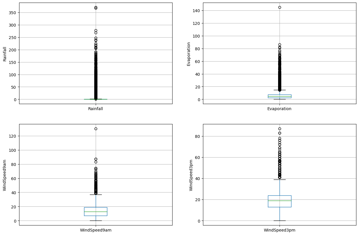
이를 통해 해당 변수들에 많은 이상값이 있음을 확인할 수 있습니다.
변수 분포 확인하기
다음 히스토그램을 통해 변수 분포를 확인하고 만약 변수가 정규 분포를 따른다면 극값 분석 (Extreme Value Analysis)을 하고, 왜도가 있는 경우에는 IQR (Interquantile range)를 찾습니다.
# plot histogram to check distribution

plture(figsize=(15,10))


plt.subplot(2, 2, 1)
fig = df.Rainfall.hist(bins=10)

fig.set_xlabel('Rainfall')
fig.set_ylabel('RainTomorrow')


plt.subplot(2, 2, 2)
fig = df.Evaporation.hist(bins=10)
fig.set_xlabel('Evaporation')
fig.set_ylabel('RainTomorrow')


plt.subplot(2, 2, 3)
fig = df.WindSpeed9am.hist(bins=10)
fig.set_xlabel('WindSpeed9am')
fig.set_ylabel('RainTomorrow')


plt.subplot(2, 2, 4)
fig = df.WindSpeed3pm.hist(bins=10)
fig.set_xlabel('WindSpeed3pm')
fig.set_ylabel('RainTomorrow')
Text(0, 0.5, 'RainTomorrow')
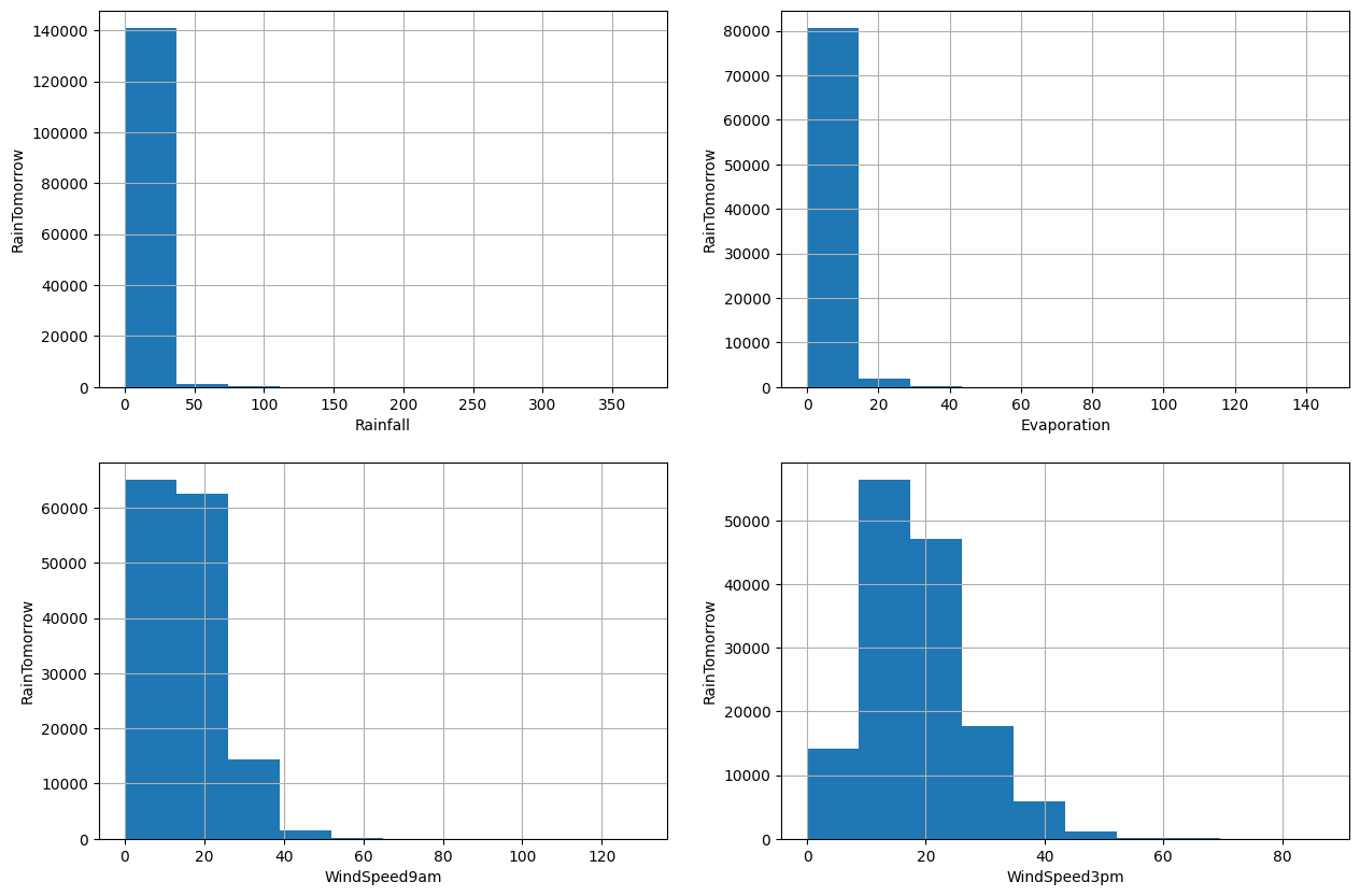
4개의 변수가 모두 왜곡되어 있음을 알 수 있습니다. 따라서 이상값을 찾기 위해 양자간 범위를 사용하겠습니다.
# find outliers for Rainfall variable

IQR = df.Rainfall.quantile(0.75) - df.Rainfall.quantile(0.25)
Lower_fence = df.Rainfall.quantile(0.25) - (IQR * 3)
Upper_fence = df.Rainfall.quantile(0.75) + (IQR * 3)
print('Rainfall outliers are values < {lowerboundary} or > {upperboundary}'.format(lowerboundary=Lower_fence, upperboundary=Upper_fence))
Rainfall outliers are values < -2.4000000000000004 or > 3.2
# find outliers for Evaporation variable

IQR = df.Evaporation.quantile(0.75) - df.Evaporation.quantile(0.25)
Lower_fence = df.Evaporation.quantile(0.25) - (IQR * 3)
Upper_fence = df.Evaporation.quantile(0.75) + (IQR * 3)
print('Evaporation outliers are values < {lowerboundary} or > {upperboundary}'.format(lowerboundary=Lower_fence, upperboundary=Upper_fence))
Evaporation outliers are values < -11.800000000000002 or > 21.800000000000004
Evaporation 변수의 최솟값과 최댓값은 각각 0.0과 145.0이므로 이상치는 21.8보다 큰 값입니다.
# find outliers for WindSpeed9am variable

IQR = df.WindSpeed9am.quantile(0.75) - df.WindSpeed9am.quantile(0.25)
Lower_fence = df.WindSpeed9am.quantile(0.25) - (IQR * 3)
Upper_fence = df.WindSpeed9am.quantile(0.75) + (IQR * 3)
print('WindSpeed9am outliers are values < {lowerboundary} or > {upperboundary}'.format(lowerboundary=Lower_fence, upperboundary=Upper_fence))
WindSpeed9am outliers are values < -29.0 or > 55.0
WindSpeed9am의 최소값과 최대값은 각각 0.0과 130.0 이므로 이상치는 값이 55.0을 초과하는 값들입니다.
# find outliers for WindSpeed3pm variable

IQR = df.WindSpeed3pm.quantile(0.75) - df.WindSpeed3pm.quantile(0.25)
Lower_fence = df.WindSpeed3pm.quantile(0.25) - (IQR * 3)
Upper_fence = df.WindSpeed3pm.quantile(0.75) + (IQR * 3)
print('WindSpeed3pm outliers are values < {lowerboundary} or > {upperboundary}'.format(lowerboundary=Lower_fence, upperboundary=Upper_fence))
WindSpeed3pm outliers are values < -20.0 or > 57.0
WindSpeed3pm 변수에서 최소값은 0.0이고 최대값은 87.0이므로 이상치는 값 > 57.0입니다.
8. 특징 벡터(feature vector) 및 타겟 변수 선언
X = df.drop(['RainTomorrow'], axis=1)

y = df['RainTomorrow']
9. 데이터를 훈련셋과 테스트셋으로 분리
!pip install -U scikit-learn
Requirement already satisfied: scikit-learn in c:\users\보일우\appdata\local\programs\python\python310\lib\site-packages (1.2.2)
Requirement already satisfied: scipy>=1.3.2 in c:\users\보일우\appdata\local\programs\python\python310\lib\site-packages (from scikit-learn) (1.10.1)
Requirement already satisfied: joblib>=1.1.1 in c:\users\보일우\appdata\local\programs\python\python310\lib\site-packages (from scikit-learn) (1.2.0)
Requirement already satisfied: numpy>=1.17.3 in c:\users\보일우\appdata\local\programs\python\python310\lib\site-packages (from scikit-learn) (1.24.2)
Requirement already satisfied: threadpoolctl>=2.0.0 in c:\users\보일우\appdata\local\programs\python\python310\lib\site-packages (from scikit-learn) (3.1.0)


[notice] A new release of pip available: 22.2.2 -> 23.1
[notice] To update, run: python.exe -m pip install --upgrade pip
# split X and y into training and testing sets

from sklearn.model_selection import train_test_split

X_train, X_test, y_train, y_test = train_test_split(X, y, test_size = 0.2, random_state = 0)
# check the shape of X_train and X_test

X_train.shape, X_test.shape
((116368, 24), (29092, 24))
10. Feature Engineering
Feature Engineering(특성 공학)은 원시 데이터(raw data)를 유용한 특성(feature)으로 변환하여 모델을 이해하고 예측력을 높이는 과정입니다.
먼저 범주형 변수와 수치형 변수를 다시 분리하여 표시합니다.
# check data types in X_train

X_train.dtypes
Location          object
MinTemp          float64
MaxTemp          float64
Rainfall         float64
Evaporation      float64
Sunshine         float64
WindGustDir       object
WindGustSpeed    float64
WindDir9am        object
WindDir3pm        object
WindSpeed9am     float64
WindSpeed3pm     float64
Humidity9am      float64
Humidity3pm      float64
Pressure9am      float64
Pressure3pm      float64
Cloud9am         float64
Cloud3pm         float64
Temp9am          float64
Temp3pm          float64
RainToday         object
Year               int32
Month              int32
Day                int32
dtype: object
# display categorical variables

categorical = [col for col in X_train.columns if X_train[col].dtypes == 'O']

categorical
['Location', 'WindGustDir', 'WindDir9am', 'WindDir3pm', 'RainToday']
# display numerical variables

numerical = [col for col in X_train.columns if X_train[col].dtypes != 'O']

numerical
['MinTemp',
 'MaxTemp',
 'Rainfall',
 'Evaporation',
 'Sunshine',
 'WindGustSpeed',
 'WindSpeed9am',
 'WindSpeed3pm',
 'Humidity9am',
 'Humidity3pm',
 'Pressure9am',
 'Pressure3pm',
 'Cloud9am',
 'Cloud3pm',
 'Temp9am',
 'Temp3pm',
 'Year',
 'Month',
 'Day']
결측값이 있는 수치형 변수에서 feature engineering을 수행합니다.
# check missing values in numerical variables in X_train

X_train[numerical].isnull().sum()
MinTemp           1183
MaxTemp           1019
Rainfall          2617
Evaporation      50355
Sunshine         55899
WindGustSpeed     8218
WindSpeed9am      1409
WindSpeed3pm      2456
Humidity9am       2147
Humidity3pm       3598
Pressure9am      12091
Pressure3pm      12064
Cloud9am         44796
Cloud3pm         47557
Temp9am           1415
Temp3pm           2865
Year                 0
Month                0
Day                  0
dtype: int64
# check missing values in numerical variables in X_test

X_test[numerical].isnull().sum()
MinTemp            302
MaxTemp            242
Rainfall           644
Evaporation      12435
Sunshine         13936
WindGustSpeed     2045
WindSpeed9am       358
WindSpeed3pm       606
Humidity9am        507
Humidity3pm        909
Pressure9am       2974
Pressure3pm       2964
Cloud9am         11092
Cloud3pm         11801
Temp9am            352
Temp3pm            744
Year                 0
Month                0
Day                  0
dtype: int64
# print percentage of missing values in the numerical variables in training set

for col in numerical:
    if X_train[col].isnull().mean()>0:
        print(col, round(X_train[col].isnull().mean(),4))
MinTemp 0.0102
MaxTemp 0.0088
Rainfall 0.0225
Evaporation 0.4327
Sunshine 0.4804
WindGustSpeed 0.0706
WindSpeed9am 0.0121
WindSpeed3pm 0.0211
Humidity9am 0.0185
Humidity3pm 0.0309
Pressure9am 0.1039
Pressure3pm 0.1037
Cloud9am 0.385
Cloud3pm 0.4087
Temp9am 0.0122
Temp3pm 0.0246
데이터가 완전히 무작위로 누락되었다고 가정합시다(MCAR). 누락된 값에 대한 대체 방법으로는 평균 또는 중앙값 대체 방법과 임의 표본 대체 방법이 있습니다. 데이터 세트에 이상치가 있는 경우 중앙값 대체 방법을 사용해야 합니다.중앙값 대체 방법은 이상치에 강건하기 때문에 중앙값 대체 방법을 사용합니다.
훈련 세트에서 적절한 통계 측정값인 중앙값을 사용하여 누락된 값을 보간합니다. 과적합을 피하기 위해 훈련 세트에서만 누락된 값 채우기에 사용될 통계 측정값은 훈련 세트에서 추출해야 합니다.
# impute missing values in X_train and X_test with respective column median in X_train

for df1 in [X_train, X_test]:
    for col in numerical:
        col_median=X_train[col].median()
        df1[col].fillna(col_median, inplace=True)
# check again missing values in numerical variables in X_train

X_train[numerical].isnull().sum()
MinTemp          0
MaxTemp          0
Rainfall         0
Evaporation      0
Sunshine         0
WindGustSpeed    0
WindSpeed9am     0
WindSpeed3pm     0
Humidity9am      0
Humidity3pm      0
Pressure9am      0
Pressure3pm      0
Cloud9am         0
Cloud3pm         0
Temp9am          0
Temp3pm          0
Year             0
Month            0
Day              0
dtype: int64
# check missing values in numerical variables in X_test

X_test[numerical].isnull().sum()
MinTemp          0
MaxTemp          0
Rainfall         0
Evaporation      0
Sunshine         0
WindGustSpeed    0
WindSpeed9am     0
WindSpeed3pm     0
Humidity9am      0
Humidity3pm      0
Pressure9am      0
Pressure3pm      0
Cloud9am         0
Cloud3pm         0
Temp9am          0
Temp3pm          0
Year             0
Month            0
Day              0
dtype: int64
이제 훈련 세트와 테스트 세트의 숫자 열에는 누락된 값이 없습니다.
결측값이 있는 범주형 변수에서 engineering을 수행
# print percentage of missing values in the categorical variables in training set

X_train[categorical].isnull().mean()
Location       0.000000
WindGustDir    0.071068
WindDir9am     0.072597
WindDir3pm     0.028951
RainToday      0.022489
dtype: float64
# print categorical variables with missing data

for col in categorical:
    if X_train[col].isnull().mean()>0:
        print(col, (X_train[col].isnull().mean()))
WindGustDir 0.07106764746322013
WindDir9am 0.07259727760208992
WindDir3pm 0.028951258077822083
RainToday 0.02248900041248453
# impute missing categorical variables with most frequent value

for df2 in [X_train, X_test]:
    df2['WindGustDir'].fillna(X_train['WindGustDir'].mode()[0], inplace=True)
    df2['WindDir9am'].fillna(X_train['WindDir9am'].mode()[0], inplace=True)
    df2['WindDir3pm'].fillna(X_train['WindDir3pm'].mode()[0], inplace=True)
    df2['RainToday'].fillna(X_train['RainToday'].mode()[0], inplace=True)
# check missing values in categorical variables in X_train

X_train[categorical].isnull().sum()
Location       0
WindGustDir    0
WindDir9am     0
WindDir3pm     0
RainToday      0
dtype: int64
# check missing values in categorical variables in X_test

X_test[categorical].isnull().sum()
Location       0
WindGustDir    0
WindDir9am     0
WindDir3pm     0
RainToday      0
dtype: int64
마지막으로 X_train과 X_test에 결측치가 있는지 확인합니다.
# check missing values in X_train

X_train.isnull().sum()
Location         0
MinTemp          0
MaxTemp          0
Rainfall         0
Evaporation      0
Sunshine         0
WindGustDir      0
WindGustSpeed    0
WindDir9am       0
WindDir3pm       0
WindSpeed9am     0
WindSpeed3pm     0
Humidity9am      0
Humidity3pm      0
Pressure9am      0
Pressure3pm      0
Cloud9am         0
Cloud3pm         0
Temp9am          0
Temp3pm          0
RainToday        0
Year             0
Month            0
Day              0
dtype: int64
# check missing values in X_test

X_test.isnull().sum()
Location         0
MinTemp          0
MaxTemp          0
Rainfall         0
Evaporation      0
Sunshine         0
WindGustDir      0
WindGustSpeed    0
WindDir9am       0
WindDir3pm       0
WindSpeed9am     0
WindSpeed3pm     0
Humidity9am      0
Humidity3pm      0
Pressure9am      0
Pressure3pm      0
Cloud9am         0
Cloud3pm         0
Temp9am          0
Temp3pm          0
RainToday        0
Year             0
Month            0
Day              0
dtype: int64
우리는 X_train과 X_test에 결측치가 없음을 확인할 수 있습니다.
수치형 변수에서 이상치 제거
우리는 Rainfall, Evaporation, WindSpeed9am 그리고 WindSpeed3pm 열이 이상치를 가지고 있다는 것을 확인했습니다. 이러한 변수에서 최댓값을 제한하고 이상치를 제거하기 위해 상위-코딩(top-coding) 접근 방식을 사용할 것입니다.
def max_value(df3, variable, top):
    return np.where(df3[variable]>top, top, df3[variable])

for df3 in [X_train, X_test]:
    df3['Rainfall'] = max_value(df3, 'Rainfall', 3.2)
    df3['Evaporation'] = max_value(df3, 'Evaporation', 21.8)
    df3['WindSpeed9am'] = max_value(df3, 'WindSpeed9am', 55)
    df3['WindSpeed3pm'] = max_value(df3, 'WindSpeed3pm', 57)
X_train.Rainfall.max(), X_test.Rainfall.max()
(3.2, 3.2)
X_train.Evaporation.max(), X_test.Evaporation.max()
(21.8, 21.8)
X_train.WindSpeed9am.max(), X_test.WindSpeed9am.max()
(55.0, 55.0)
X_train.WindSpeed3pm.max(), X_test.WindSpeed3pm.max()
(57.0, 57.0)
X_train[numerical].describe()
| MinTemp | MaxTemp | Rainfall | Evaporation | Sunshine | WindGustSpeed | WindSpeed9am | WindSpeed3pm | Humidity9am | Humidity3pm | Pressure9am | Pressure3pm | Cloud9am | Cloud3pm | Temp9am | Temp3pm | Year | Month | Day | |
|---|---|---|---|---|---|---|---|---|---|---|---|---|---|---|---|---|---|---|---|
| count | 116368.000000 | 116368.000000 | 116368.000000 | 116368.000000 | 116368.000000 | 116368.000000 | 116368.000000 | 116368.000000 | 116368.000000 | 116368.000000 | 116368.000000 | 116368.000000 | 116368.000000 | 116368.000000 | 116368.000000 | 116368.000000 | 116368.000000 | 116368.000000 | 116368.000000 |
| mean | 12.190189 | 23.203107 | 0.670800 | 5.093362 | 7.982476 | 39.982091 | 14.029381 | 18.687466 | 68.950691 | 51.605828 | 1017.639891 | 1015.244946 | 4.664092 | 4.710728 | 16.979454 | 21.657195 | 2012.767058 | 6.395091 | 15.731954 |
| std | 6.366893 | 7.085408 | 1.181512 | 2.800200 | 2.761639 | 13.127953 | 8.835596 | 8.700618 | 18.811437 | 20.439999 | 6.728234 | 6.661517 | 2.280687 | 2.106040 | 6.449641 | 6.848293 | 2.538401 | 3.425451 | 8.796931 |
| min | -8.500000 | -4.800000 | 0.000000 | 0.000000 | 0.000000 | 6.000000 | 0.000000 | 0.000000 | 0.000000 | 0.000000 | 980.500000 | 977.100000 | 0.000000 | 0.000000 | -7.200000 | -5.400000 | 2007.000000 | 1.000000 | 1.000000 |
| 25% | 7.700000 | 18.000000 | 0.000000 | 4.000000 | 8.200000 | 31.000000 | 7.000000 | 13.000000 | 57.000000 | 37.000000 | 1013.500000 | 1011.100000 | 3.000000 | 4.000000 | 12.300000 | 16.700000 | 2011.000000 | 3.000000 | 8.000000 |
| 50% | 12.000000 | 22.600000 | 0.000000 | 4.700000 | 8.400000 | 39.000000 | 13.000000 | 19.000000 | 70.000000 | 52.000000 | 1017.600000 | 1015.200000 | 5.000000 | 5.000000 | 16.700000 | 21.100000 | 2013.000000 | 6.000000 | 16.000000 |
| 75% | 16.800000 | 28.200000 | 0.600000 | 5.200000 | 8.600000 | 46.000000 | 19.000000 | 24.000000 | 83.000000 | 65.000000 | 1021.800000 | 1019.400000 | 6.000000 | 6.000000 | 21.500000 | 26.200000 | 2015.000000 | 9.000000 | 23.000000 |
| max | 31.900000 | 48.100000 | 3.200000 | 21.800000 | 14.500000 | 135.000000 | 55.000000 | 57.000000 | 100.000000 | 100.000000 | 1041.000000 | 1039.600000 | 9.000000 | 8.000000 | 40.200000 | 46.700000 | 2017.000000 | 12.000000 | 31.000000 |
Rainfall, Evaporation, WindSpeed9am, WindSpeed3pm 열의 이상치가 상한선으로 대체된 것을 볼 수 있습니다.
범주형 변수 인코딩
categorical
['Location', 'WindGustDir', 'WindDir9am', 'WindDir3pm', 'RainToday']
X_train[categorical].head()
| Location | WindGustDir | WindDir9am | WindDir3pm | RainToday | |
|---|---|---|---|---|---|
| 22926 | NorfolkIsland | ESE | ESE | ESE | No |
| 80735 | Watsonia | NE | NNW | NNE | No |
| 121764 | Perth | SW | N | SW | Yes |
| 139821 | Darwin | ESE | ESE | E | No |
| 1867 | Albury | E | ESE | E | Yes |
pip install category-encoders
Requirement already satisfied: category-encoders in c:\users\보일우\appdata\local\programs\python\python310\lib\site-packages (2.6.0)
Requirement already satisfied: numpy>=1.14.0 in c:\users\보일우\appdata\local\programs\python\python310\lib\site-packages (from category-encoders) (1.24.2)
Requirement already satisfied: patsy>=0.5.1 in c:\users\보일우\appdata\local\programs\python\python310\lib\site-packages (from category-encoders) (0.5.3)
Requirement already satisfied: pandas>=1.0.5 in c:\users\보일우\appdata\local\programs\python\python310\lib\site-packages (from category-encoders) (2.0.0)
Requirement already satisfied: scipy>=1.0.0 in c:\users\보일우\appdata\local\programs\python\python310\lib\site-packages (from category-encoders) (1.10.1)
Requirement already satisfied: scikit-learn>=0.20.0 in c:\users\보일우\appdata\local\programs\python\python310\lib\site-packages (from category-encoders) (1.2.2)
Requirement already satisfied: statsmodels>=0.9.0 in c:\users\보일우\appdata\local\programs\python\python310\lib\site-packages (from category-encoders) (0.13.5)
Requirement already satisfied: pytz>=2020.1 in c:\users\보일우\appdata\local\programs\python\python310\lib\site-packages (from pandas>=1.0.5->category-encoders) (2023.3)
Requirement already satisfied: tzdata>=2022.1 in c:\users\보일우\appdata\local\programs\python\python310\lib\site-packages (from pandas>=1.0.5->category-encoders) (2023.3)
Requirement already satisfied: python-dateutil>=2.8.2 in c:\users\보일우\appdata\local\programs\python\python310\lib\site-packages (from pandas>=1.0.5->category-encoders) (2.8.2)
Requirement already satisfied: six in c:\users\보일우\appdata\local\programs\python\python310\lib\site-packages (from patsy>=0.5.1->category-encoders) (1.16.0)
Requirement already satisfied: threadpoolctl>=2.0.0 in c:\users\보일우\appdata\local\programs\python\python310\lib\site-packages (from scikit-learn>=0.20.0->category-encoders) (3.1.0)
Requirement already satisfied: joblib>=1.1.1 in c:\users\보일우\appdata\local\programs\python\python310\lib\site-packages (from scikit-learn>=0.20.0->category-encoders) (1.2.0)
Requirement already satisfied: packaging>=21.3 in c:\users\보일우\appdata\local\programs\python\python310\lib\site-packages (from statsmodels>=0.9.0->category-encoders) (23.0)
Note: you may need to restart the kernel to use updated packages.


[notice] A new release of pip available: 22.2.2 -> 23.1
[notice] To update, run: python.exe -m pip install --upgrade pip
# encode RainToday variable

import category_encoders as ce

encoder = ce.BinaryEncoder(cols=['RainToday'])

X_train = encoder.fit_transform(X_train)

X_test = encoder.transform(X_test)
X_train.head()
| Location | MinTemp | MaxTemp | Rainfall | Evaporation | Sunshine | WindGustDir | WindGustSpeed | WindDir9am | WindDir3pm | ... | Pressure3pm | Cloud9am | Cloud3pm | Temp9am | Temp3pm | RainToday_0 | RainToday_1 | Year | Month | Day | |
|---|---|---|---|---|---|---|---|---|---|---|---|---|---|---|---|---|---|---|---|---|---|
| 22926 | NorfolkIsland | 18.8 | 23.7 | 0.2 | 5.0 | 7.3 | ESE | 52.0 | ESE | ESE | ... | 1013.9 | 5.0 | 7.0 | 21.4 | 22.2 | 0 | 1 | 2014 | 3 | 12 |
| 80735 | Watsonia | 9.3 | 24.0 | 0.2 | 1.6 | 10.9 | NE | 48.0 | NNW | NNE | ... | 1014.6 | 3.0 | 5.0 | 14.3 | 23.2 | 0 | 1 | 2016 | 10 | 6 |
| 121764 | Perth | 10.9 | 22.2 | 1.4 | 1.2 | 9.6 | SW | 26.0 | N | SW | ... | 1014.9 | 1.0 | 2.0 | 16.6 | 21.5 | 1 | 0 | 2011 | 8 | 31 |
| 139821 | Darwin | 19.3 | 29.9 | 0.0 | 9.2 | 11.0 | ESE | 43.0 | ESE | E | ... | 1012.1 | 1.0 | 1.0 | 23.2 | 29.1 | 0 | 1 | 2010 | 6 | 11 |
| 1867 | Albury | 15.7 | 17.6 | 3.2 | 4.7 | 8.4 | E | 20.0 | ESE | E | ... | 1010.5 | 8.0 | 8.0 | 16.5 | 17.3 | 1 | 0 | 2014 | 4 | 10 |
5 rows × 25 columns
RainToday 변수에서 추가적인 변수인 RainToday_0과 RainToday_1이 생성된 것을 볼 수 있습니다.
이제, X_train training set을 생성하겠습니다.
X_train = pd.concat([X_train[numerical], X_train[['RainToday_0', 'RainToday_1']],
                     pd.get_dummies(X_train.Location),
                     pd.get_dummies(X_train.WindGustDir),
                     pd.get_dummies(X_train.WindDir9am),
                     pd.get_dummies(X_train.WindDir3pm)], axis=1)
X_train.head()
| MinTemp | MaxTemp | Rainfall | Evaporation | Sunshine | WindGustSpeed | WindSpeed9am | WindSpeed3pm | Humidity9am | Humidity3pm | ... | NNW | NW | S | SE | SSE | SSW | SW | W | WNW | WSW | |
|---|---|---|---|---|---|---|---|---|---|---|---|---|---|---|---|---|---|---|---|---|---|
| 22926 | 18.8 | 23.7 | 0.2 | 5.0 | 7.3 | 52.0 | 31.0 | 28.0 | 74.0 | 73.0 | ... | False | False | False | False | False | False | False | False | False | False |
| 80735 | 9.3 | 24.0 | 0.2 | 1.6 | 10.9 | 48.0 | 13.0 | 24.0 | 74.0 | 55.0 | ... | False | False | False | False | False | False | False | False | False | False |
| 121764 | 10.9 | 22.2 | 1.4 | 1.2 | 9.6 | 26.0 | 0.0 | 11.0 | 85.0 | 47.0 | ... | False | False | False | False | False | False | True | False | False | False |
| 139821 | 19.3 | 29.9 | 0.0 | 9.2 | 11.0 | 43.0 | 26.0 | 17.0 | 44.0 | 37.0 | ... | False | False | False | False | False | False | False | False | False | False |
| 1867 | 15.7 | 17.6 | 3.2 | 4.7 | 8.4 | 20.0 | 11.0 | 13.0 | 100.0 | 100.0 | ... | False | False | False | False | False | False | False | False | False | False |
5 rows × 118 columns
X_test 테스트 세트를 만들겠습니다.
X_test = pd.concat([X_test[numerical], X_test[['RainToday_0', 'RainToday_1']],
                     pd.get_dummies(X_test.Location),
                     pd.get_dummies(X_test.WindGustDir),
                     pd.get_dummies(X_test.WindDir9am),
                     pd.get_dummies(X_test.WindDir3pm)], axis=1)
X_test.head()
| MinTemp | MaxTemp | Rainfall | Evaporation | Sunshine | WindGustSpeed | WindSpeed9am | WindSpeed3pm | Humidity9am | Humidity3pm | ... | NNW | NW | S | SE | SSE | SSW | SW | W | WNW | WSW | |
|---|---|---|---|---|---|---|---|---|---|---|---|---|---|---|---|---|---|---|---|---|---|
| 138175 | 21.9 | 39.4 | 1.6 | 11.2 | 11.5 | 57.0 | 20.0 | 33.0 | 50.0 | 26.0 | ... | False | False | False | False | False | False | False | False | False | False |
| 38638 | 20.5 | 37.5 | 0.0 | 9.2 | 8.4 | 59.0 | 17.0 | 20.0 | 47.0 | 22.0 | ... | False | False | False | False | False | False | False | False | False | False |
| 124058 | 5.1 | 17.2 | 0.2 | 4.7 | 8.4 | 50.0 | 28.0 | 22.0 | 68.0 | 51.0 | ... | False | False | False | False | False | False | False | True | False | False |
| 99214 | 11.9 | 16.8 | 1.0 | 4.7 | 8.4 | 28.0 | 11.0 | 13.0 | 80.0 | 79.0 | ... | False | False | False | False | False | False | True | False | False | False |
| 25097 | 7.5 | 21.3 | 0.0 | 4.7 | 8.4 | 15.0 | 2.0 | 7.0 | 88.0 | 52.0 | ... | False | False | False | False | False | False | False | False | False | False |
5 rows × 118 columns
모델 구축을 위해 훈련 및 테스트 세트를 준비했습니다. 그러나 그 전에, 모든 특성 변수를 동일한 척도로 매핑하는 스케일링을 합니다.
11. 특성 스케일링 (Feature Scaling)
X_train.describe()
| MinTemp | MaxTemp | Rainfall | Evaporation | Sunshine | WindGustSpeed | WindSpeed9am | WindSpeed3pm | Humidity9am | Humidity3pm | ... | Pressure3pm | Cloud9am | Cloud3pm | Temp9am | Temp3pm | Year | Month | Day | RainToday_0 | RainToday_1 | |
|---|---|---|---|---|---|---|---|---|---|---|---|---|---|---|---|---|---|---|---|---|---|
| count | 116368.000000 | 116368.000000 | 116368.000000 | 116368.000000 | 116368.000000 | 116368.000000 | 116368.000000 | 116368.000000 | 116368.000000 | 116368.000000 | ... | 116368.000000 | 116368.000000 | 116368.000000 | 116368.000000 | 116368.000000 | 116368.000000 | 116368.000000 | 116368.000000 | 116368.000000 | 116368.000000 |
| mean | 12.190189 | 23.203107 | 0.670800 | 5.093362 | 7.982476 | 39.982091 | 14.029381 | 18.687466 | 68.950691 | 51.605828 | ... | 1015.244946 | 4.664092 | 4.710728 | 16.979454 | 21.657195 | 2012.767058 | 6.395091 | 15.731954 | 0.219648 | 0.780352 |
| std | 6.366893 | 7.085408 | 1.181512 | 2.800200 | 2.761639 | 13.127953 | 8.835596 | 8.700618 | 18.811437 | 20.439999 | ... | 6.661517 | 2.280687 | 2.106040 | 6.449641 | 6.848293 | 2.538401 | 3.425451 | 8.796931 | 0.414010 | 0.414010 |
| min | -8.500000 | -4.800000 | 0.000000 | 0.000000 | 0.000000 | 6.000000 | 0.000000 | 0.000000 | 0.000000 | 0.000000 | ... | 977.100000 | 0.000000 | 0.000000 | -7.200000 | -5.400000 | 2007.000000 | 1.000000 | 1.000000 | 0.000000 | 0.000000 |
| 25% | 7.700000 | 18.000000 | 0.000000 | 4.000000 | 8.200000 | 31.000000 | 7.000000 | 13.000000 | 57.000000 | 37.000000 | ... | 1011.100000 | 3.000000 | 4.000000 | 12.300000 | 16.700000 | 2011.000000 | 3.000000 | 8.000000 | 0.000000 | 1.000000 |
| 50% | 12.000000 | 22.600000 | 0.000000 | 4.700000 | 8.400000 | 39.000000 | 13.000000 | 19.000000 | 70.000000 | 52.000000 | ... | 1015.200000 | 5.000000 | 5.000000 | 16.700000 | 21.100000 | 2013.000000 | 6.000000 | 16.000000 | 0.000000 | 1.000000 |
| 75% | 16.800000 | 28.200000 | 0.600000 | 5.200000 | 8.600000 | 46.000000 | 19.000000 | 24.000000 | 83.000000 | 65.000000 | ... | 1019.400000 | 6.000000 | 6.000000 | 21.500000 | 26.200000 | 2015.000000 | 9.000000 | 23.000000 | 0.000000 | 1.000000 |
| max | 31.900000 | 48.100000 | 3.200000 | 21.800000 | 14.500000 | 135.000000 | 55.000000 | 57.000000 | 100.000000 | 100.000000 | ... | 1039.600000 | 9.000000 | 8.000000 | 40.200000 | 46.700000 | 2017.000000 | 12.000000 | 31.000000 | 1.000000 | 1.000000 |
8 rows × 21 columns
cols = X_train.columns
from sklearn.preprocessing import MinMaxScaler

scaler = MinMaxScaler()

X_train = scaler.fit_transform(X_train)

X_test = scaler.transform(X_test)
X_train = pd.DataFrame(X_train, columns=[cols])
X_test = pd.DataFrame(X_test, columns=[cols])
X_train.describe()
| MinTemp | MaxTemp | Rainfall | Evaporation | Sunshine | WindGustSpeed | WindSpeed9am | WindSpeed3pm | Humidity9am | Humidity3pm | ... | NNW | NW | S | SE | SSE | SSW | SW | W | WNW | WSW | |
|---|---|---|---|---|---|---|---|---|---|---|---|---|---|---|---|---|---|---|---|---|---|
| count | 116368.000000 | 116368.000000 | 116368.000000 | 116368.000000 | 116368.000000 | 116368.000000 | 116368.000000 | 116368.000000 | 116368.000000 | 116368.000000 | ... | 116368.000000 | 116368.000000 | 116368.000000 | 116368.000000 | 116368.000000 | 116368.000000 | 116368.000000 | 116368.000000 | 116368.000000 | 116368.000000 |
| mean | 0.512133 | 0.529359 | 0.209625 | 0.233640 | 0.550516 | 0.263427 | 0.255080 | 0.327850 | 0.689507 | 0.516058 | ... | 0.054078 | 0.059123 | 0.068447 | 0.103723 | 0.065224 | 0.056055 | 0.064786 | 0.069323 | 0.060309 | 0.064958 |
| std | 0.157596 | 0.133940 | 0.369223 | 0.128450 | 0.190458 | 0.101767 | 0.160647 | 0.152642 | 0.188114 | 0.204400 | ... | 0.226173 | 0.235855 | 0.252512 | 0.304902 | 0.246922 | 0.230029 | 0.246149 | 0.254004 | 0.238059 | 0.246452 |
| min | 0.000000 | 0.000000 | 0.000000 | 0.000000 | 0.000000 | 0.000000 | 0.000000 | 0.000000 | 0.000000 | 0.000000 | ... | 0.000000 | 0.000000 | 0.000000 | 0.000000 | 0.000000 | 0.000000 | 0.000000 | 0.000000 | 0.000000 | 0.000000 |
| 25% | 0.400990 | 0.431002 | 0.000000 | 0.183486 | 0.565517 | 0.193798 | 0.127273 | 0.228070 | 0.570000 | 0.370000 | ... | 0.000000 | 0.000000 | 0.000000 | 0.000000 | 0.000000 | 0.000000 | 0.000000 | 0.000000 | 0.000000 | 0.000000 |
| 50% | 0.507426 | 0.517958 | 0.000000 | 0.215596 | 0.579310 | 0.255814 | 0.236364 | 0.333333 | 0.700000 | 0.520000 | ... | 0.000000 | 0.000000 | 0.000000 | 0.000000 | 0.000000 | 0.000000 | 0.000000 | 0.000000 | 0.000000 | 0.000000 |
| 75% | 0.626238 | 0.623819 | 0.187500 | 0.238532 | 0.593103 | 0.310078 | 0.345455 | 0.421053 | 0.830000 | 0.650000 | ... | 0.000000 | 0.000000 | 0.000000 | 0.000000 | 0.000000 | 0.000000 | 0.000000 | 0.000000 | 0.000000 | 0.000000 |
| max | 1.000000 | 1.000000 | 1.000000 | 1.000000 | 1.000000 | 1.000000 | 1.000000 | 1.000000 | 1.000000 | 1.000000 | ... | 1.000000 | 1.000000 | 1.000000 | 1.000000 | 1.000000 | 1.000000 | 1.000000 | 1.000000 | 1.000000 | 1.000000 |
8 rows × 118 columns
Logistic Regression 분류기에 입력할 수 있는 X_train 데이터셋이 준비되었습니다.
12. 모델훈련
sklearn 사용 중단으로 인해 구현해야하는 주요 수정 사항이 있으며 누락 된 값을 채운 다음 y_train 및 y_test 인코딩합니다.
from sklearn.preprocessing import LabelEncoder

y_train = pd.DataFrame(y_train)
y_test = pd.DataFrame(y_test)

y_train['RainTomorrow'].fillna(y_train['RainTomorrow'].mode()[0], inplace=True)
y_test['RainTomorrow'].fillna(y_test['RainTomorrow'].mode()[0], inplace=True)

train_le = LabelEncoder()
test_le = LabelEncoder()

train_le.fit(y_train['RainTomorrow'].astype('str').drop_duplicates())
test_le.fit(y_test['RainTomorrow'].astype('str').drop_duplicates())

y_train['enc'] = train_le.transform(y_train['RainTomorrow'].astype('str'))
y_test['enc'] = train_le.transform(y_test['RainTomorrow'].astype('str'))

y_train.drop(columns=['RainTomorrow'], inplace=True)
y_test.drop(columns=['RainTomorrow'], inplace=True)
# train a logistic regression model on the training set
from sklearn.linear_model import LogisticRegression


# instantiate the model
logreg = LogisticRegression(solver='liblinear', random_state=0)


# fit the model
logreg.fit(X_train, y_train)
LogisticRegression(random_state=0, solver='liblinear')In a Jupyter environment, please rerun this cell to show the HTML representation or trust the notebook.
On GitHub, the HTML representation is unable to render, please try loading this page with nbviewer.org.
LogisticRegression(random_state=0, solver='liblinear')
13. 결과 예측
y_pred_test = logreg.predict(X_test)

y_pred_test
array([0, 0, 0, ..., 1, 0, 0])
predict_proba 메서드
predict_proba 메서드는 배열 형태로 해당 경우의 타겟 변수(0과 1)에 대한 확률을 제공합니다.
0은 비가 오지 않을 확률을, 1은 비가 올 확률을 나타냅니다.
# probability of getting output as 0 - no rain

logreg.predict_proba(X_test)[:,0]
array([0.83217211, 0.74550754, 0.79860594, ..., 0.42025779, 0.65752483,
       0.96955092])
# probability of getting output as 1 - rain

logreg.predict_proba(X_test)[:,1]
array([0.16782789, 0.25449246, 0.20139406, ..., 0.57974221, 0.34247517,
       0.03044908])
14. 정확도 확인
from sklearn.metrics import accuracy_score

print('Model accuracy score: {0:0.4f}'. format(accuracy_score(y_test, y_pred_test)))
Model accuracy score: 0.8484
y_test는 실제 클래스 레이블이며, y_pred_test는 테스트 세트에서 예측된 클래스 레이블입니다.
이제 과적합을 확인하기 위해 학습 세트와 테스트 세트 정확도를 비교하겠습니다.
y_pred_train = logreg.predict(X_train)

y_pred_train
array([0, 0, 0, ..., 0, 0, 0])
print('Training-set accuracy score: {0:0.4f}'. format(accuracy_score(y_train, y_pred_train)))
Training-set accuracy score: 0.8488
과적합(overfitting)과 과소적합(underfitting) 확인하기
# print the scores on training and test set

print('Training set score: {:.4f}'.format(logreg.score(X_train, y_train)))

print('Test set score: {:.4f}'.format(logreg.score(X_test, y_test)))
Training set score: 0.8488
Test set score: 0.8484
학습 세트 정확도 점수는 0.8488이고 테스트 세트 정확도는 0.8484입니다. 이 두 값은 매우 유사합니다. 따라서, 과적합 문제는 없습니다.
로지스틱 회귀에서 C의 기본값은 1입니다. 이 값은 학습 세트와 테스트 세트 모두 약 85%의 정확도로 좋은 성능을 제공합니다. 그러나 학습 세트와 테스트 세트의 모델 성능이 매우 유사하므로 과소적합의 가능성이 있습니다.
따라서 C 값을 높여 더 유연한 모델을 학습시킵니다.
# fit the Logsitic Regression model with C=100

# instantiate the model
logreg100 = LogisticRegression(C=100, solver='liblinear', random_state=0)


# fit the model
logreg100.fit(X_train, y_train)
LogisticRegression(C=100, random_state=0, solver='liblinear')In a Jupyter environment, please rerun this cell to show the HTML representation or trust the notebook.
On GitHub, the HTML representation is unable to render, please try loading this page with nbviewer.org.
LogisticRegression(C=100, random_state=0, solver='liblinear')
# print the scores on training and test set

print('Training set score: {:.4f}'.format(logreg100.score(X_train, y_train)))

print('Test set score: {:.4f}'.format(logreg100.score(X_test, y_test)))
Training set score: 0.8489
Test set score: 0.8492
우리는 C=100을 사용하면 테스트 세트 정확도가 높아지고 약간의 훈련 세트 정확도 증가도 볼 수 있습니다. 그러므로 더 복잡한 모델이 더 나은 성능을 발휘할 것으로 결론지을 수 있습니다.
이제 C=1의 기본값보다 더 규제가 강한 모델을 사용할 때, 즉 C=0.01로 더 많이 규제된 모델을 사용하면 기본 매개변수에 비해 학습 및 테스트 세트의 정확도가 감소합니다.
# fit the Logsitic Regression model with C=001

# instantiate the model
logreg001 = LogisticRegression(C=0.01, solver='liblinear', random_state=0)


# fit the model
logreg001.fit(X_train, y_train)
LogisticRegression(C=0.01, random_state=0, solver='liblinear')In a Jupyter environment, please rerun this cell to show the HTML representation or trust the notebook.
On GitHub, the HTML representation is unable to render, please try loading this page with nbviewer.org.
LogisticRegression(C=0.01, random_state=0, solver='liblinear')
# print the scores on training and test set

print('Training set score: {:.4f}'.format(logreg001.score(X_train, y_train)))

print('Test set score: {:.4f}'.format(logreg001.score(X_test, y_test)))
Training set score: 0.8427
Test set score: 0.8418
모델의 정확도를 NULL 정확도와 비교
그래서 모델 정확도는 0.8484입니다. 하지만 위의 정확도만으로는 모델이 매우 좋다고 말할 수 없습니다. 널(nul) 정확도와 비교해야 합니다. 널 정확도는 가장 빈번하게 나타나는 클래스를 항상 예측하는 것으로 얻을 수 있는 정확도입니다.
그러므로 먼저 테스트 세트에서 클래스 분포를 확인해야 합니다.
# check class distribution in test set

y_test.value_counts()
enc
0      22726
1       6366
Name: count, dtype: int64
# check null accuracy score

null_accuracy = (22067/(22067+6372))

print('Null accuracy score: {0:0.4f}'. format(null_accuracy))
Null accuracy score: 0.7759
우리는 우리의 모델 정확도 점수가 0.8484인 반면 널 정확도 점수는 0.7759임을 알 수 있습니다. 따라서, 우리는 우리의 로지스틱 회귀 모델이 클래스 레이블을 예측하는 데 아주 좋은 성능을 발휘하고 있다고 결론지을 수 있습니다.
이제 위의 분석을 기반으로, 우리는 분류 모델의 정확도가 매우 좋다는 결론을 내릴 수 있습니다. 우리 모델은 클래스 레이블을 예측하는 데 아주 잘하고 있습니다.
하지만, 이는 값의 분포를 제공하지 않으며, 분류기가 어떤 유형의 오류를 만들고 있는지에 대해 알려주지 않습니다.
이를 위해 우리는 혼동 행렬(Confusion matrix)이라는 도구를 사용할 수 있습니다.
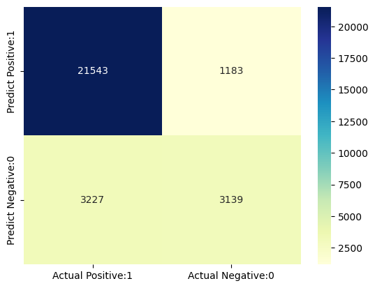
15.혼동 행렬(Confusion matrix)
혼동 행렬(confusion matrix)은 분류 모델의 성능 및 모델이 만드는 오류 유형에 대한 명확한 그림을 제공하고 각 범주별로 올바른 및 부정확한 예측을 요약합니다. 이 요약은 표 형태로 나타납니다.
분류 모델 성능을 평가할 때 네 가지 결과는 아래와 같습니다.
True Positives (TP) - True Positives는 관측값이 특정 클래스에 속하고 실제로도 해당 클래스에 속한 경우 발생
True Negatives (TN) - True Negatives는 관측값이 특정 클래스에 속하지 않고 실제로도 해당 클래스에 속하지 않은 경우 발생.
False Positives (FP) - False Positives는 관측값이 특정 클래스에 속한다고 예측하지만, 실제로는 해당 클래스에 속하지 않은 경우 발생 / 1종 오류(Type I error)
False Negatives (FN) - False Negatives는 관측값이 특정 클래스에 속하지 않는다고 예측하지만, 실제로는 해당 클래스에 속한 경우 발생 / 이는 매우 심각한 오류이며, 2종 오류(Type II error)
네 가지 결과 혼동 행렬 요약
# Print the Confusion Matrix and slice it into four pieces

from sklearn.metrics import confusion_matrix

cm = confusion_matrix(y_test, y_pred_test)

print('Confusion matrix\n\n', cm)

print('\nTrue Positives(TP) = ', cm[0,0])

print('\nTrue Negatives(TN) = ', cm[1,1])

print('\nFalse Positives(FP) = ', cm[0,1])

print('\nFalse Negatives(FN) = ', cm[1,0])
Confusion matrix

 [[21543  1183]
 [ 3227  3139]]

True Positives(TP) =  21543

True Negatives(TN) =  3139

False Positives(FP) =  1183

False Negatives(FN) =  3227
위의 혼동 행렬은 20892 + 3285 = 24177개의 정확한 예측과 3087 + 1175 = 4262개의 잘못된 예측을 보여줍니다.
- True Positives (실제 Positive:1 및 예측 Positive:1) - 21543
- True Negatives (실제 Negative:0 및 예측 Negative:0) - 3139
- False Positives (실제 Negative:0 및 예측 Positive:1) - 1183 (Type I 오류)
- False Negatives (실제 Positive:1 및 예측 Negative:0) - 3227 (Type II 오류)
# visualize confusion matrix with seaborn heatmap

cm_matrix = pd.DataFrame(data=cm, columns=['Actual Positive:1', 'Actual Negative:0'],
                                 index=['Predict Positive:1', 'Predict Negative:0'])

sns.heatmap(cm_matrix, annot=True, fmt='d', cmap='YlGnBu')
<Axes: >
16. 분류 성능 평가 지표
분류 보고서(Classification Report)
분류 보고서는 분류 모델의 성능을 평가하는 또 다른 방법입니다. 분류 모델의 정밀도(precision), 재현율(recall), f1 점수 및 지원(support) 점수를 나타냅니다.
분류 보고서는 다음과 같이 출력할 수 있습니다.
from sklearn.metrics import classification_report

print(classification_report(y_test, y_pred_test))
              precision    recall  f1-score   support

           0       0.87      0.95      0.91     22726
           1       0.73      0.49      0.59      6366

    accuracy                           0.85     29092
   macro avg       0.80      0.72      0.75     29092
weighted avg       0.84      0.85      0.84     29092
분류 정확도(Classification accuracy)
TP = cm[0,0]
TN = cm[1,1]
FP = cm[0,1]
FN = cm[1,0]
# print classification accuracy

classification_accuracy = (TP + TN) / float(TP + TN + FP + FN)

print('Classification accuracy : {0:0.4f}'.format(classification_accuracy))
Classification accuracy : 0.8484
분류 오차(Classification error)
# print classification error

classification_error = (FP + FN) / float(TP + TN + FP + FN)

print('Classification error : {0:0.4f}'.format(classification_error))
Classification error : 0.1516
Precision(정밀도)
정밀도(Precision)는 예측된 양성 중 올바르게 예측된 비율을 의미합니다. 이는 진짜 양성(True Positive, TP)의 수를 예측된 양성(True Positive, TP)과 예측된 양성(False Positive, FP)의 합으로 나눈 비율입니다.
수학적으로는 정밀도는 TP를 (TP + FP)로 나눈 비율로 정의될 수 있습니다.
# print precision score

precision = TP / float(TP + FP)


print('Precision : {0:0.4f}'.format(precision))
Precision : 0.9479
Recall
민감도(Sensitivity)로도 불리는 Recall은 실제 양성인 것 중에서 올바르게 예측한 비율을 나타냅니다. 진짜 양성(TP)을 실제 양성(TP + FN)의 합으로 나눈 비율로 표현됩니다.
수학적으로 Recall은 TP를 (TP + FN)으로 나눈 비율로 정의될 수 있습니다.
recall = TP / float(TP + FN)

print('Recall or Sensitivity : {0:0.4f}'.format(recall))
Recall or Sensitivity : 0.8697
True Positive Rate (TPR)
True Positive Rate (TPR)는 Recall과 동의어입니다.
true_positive_rate = TP / float(TP + FN)


print('True Positive Rate : {0:0.4f}'.format(true_positive_rate))
True Positive Rate : 0.8697
False Positive Rate(FPR)
false_positive_rate = FP / float(FP + TN)


print('False Positive Rate : {0:0.4f}'.format(false_positive_rate))
False Positive Rate : 0.2737
Specificity
specificity = TN / (TN + FP)

print('Specificity : {0:0.4f}'.format(specificity))
Specificity : 0.7263
f1-score
f1-score는 정밀도와 재현율의 가중 조화 평균입니다. 최상의 f1-score는 1.0이며, 최악의 경우는 0.0입니다. f1-점수는 정밀도와 재현율의 조화 평균이므로, f1-score는 정확도 측정보다 항상 낮습니다. 이는 정확도 측정이 정밀도와 재현율을 포함하기 때문입니다. 분류기 모델을 비교할 때는 f1-score의 가중 평균을 사용해야 하며, 전체 정확도보다 이 지표를 더욱 중요시해야 합니다.
Support
Support는 데이터셋에서 해당 클래스의 실제 발생 횟수입니다.
17. 임계값 조정
# print the first 10 predicted probabilities of two classes- 0 and 1

y_pred_prob = logreg.predict_proba(X_test)[0:10]

y_pred_prob
array([[0.83217211, 0.16782789],
       [0.74550754, 0.25449246],
       [0.79860594, 0.20139406],
       [0.58506456, 0.41493544],
       [0.92162871, 0.07837129],
       [0.95626453, 0.04373547],
       [0.57882814, 0.42117186],
       [0.50298442, 0.49701558],
       [0.80278354, 0.19721646],
       [0.72342399, 0.27657601]])
관측 결과
-
각 행에서의 숫자들은 1로 합쳐짐
-
2개의 열은 각각 0과 1이라는 두 개의 클래스에 해당
-
클래스 0 - 내일 비가 오지 않을 확률에 대한 예측 확률
-
클래스 1 - 내일 비가 올 확률에 대한 예측 확률
-
-
예측 확률의 중요성
- 우리는 비나 비가 오지 않을 확률에 따라 관측값들을 순위를 매길 수 있음
-
predict_proba 과정
-
확률을 예측
-
가장 높은 확률을 가진 클래스를 선택
-
-
분류 임계값
-
0.5의 분류 임계값
-
확률 > 0.5인 경우, 클래스 1 - 비가 올 확률이 예측
-
확률 < 0.5인 경우, 클래스 0 - 비가 오지 않을 확률이 예측
-
# store the probabilities in dataframe

y_pred_prob_df = pd.DataFrame(data=y_pred_prob, columns=['Prob of - No rain tomorrow (0)', 'Prob of - Rain tomorrow (1)'])

y_pred_prob_df
| Prob of - No rain tomorrow (0) | Prob of - Rain tomorrow (1) | |
|---|---|---|
| 0 | 0.832172 | 0.167828 |
| 1 | 0.745508 | 0.254492 |
| 2 | 0.798606 | 0.201394 |
| 3 | 0.585065 | 0.414935 |
| 4 | 0.921629 | 0.078371 |
| 5 | 0.956265 | 0.043735 |
| 6 | 0.578828 | 0.421172 |
| 7 | 0.502984 | 0.497016 |
| 8 | 0.802784 | 0.197216 |
| 9 | 0.723424 | 0.276576 |
# print the first 10 predicted probabilities for class 1 - Probability of rain

logreg.predict_proba(X_test)[0:10, 1]
array([0.16782789, 0.25449246, 0.20139406, 0.41493544, 0.07837129,
       0.04373547, 0.42117186, 0.49701558, 0.19721646, 0.27657601])
# store the predicted probabilities for class 1 - Probability of rain

y_pred1 = logreg.predict_proba(X_test)[:, 1]
# plot histogram of predicted probabilities


# adjust the font size
plt.rcParams['font.size'] = 12


# plot histogram with 10 bins
plt.hist(y_pred1, bins = 10)


# set the title of predicted probabilities
plt.title('Histogram of predicted probabilities of rain')


# set the x-axis limit
plt.xlim(0,1)


# set the title
plt.xlabel('Predicted probabilities of rain')
plt.ylabel('Frequency')
Text(0, 0.5, 'Frequency')
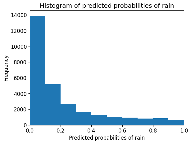
관측 결과
- 위의 히스토그램은 매우 양의 왜도를 보임
- 첫 번째 열은 0.0과 0.1 사이의 확률을 갖는 관측치가 약 15,000개 있음
- 확률이 0.5보다 큰 관측치는 적음
- 따라서 이 소수의 관측치는 내일 비가 올 것으로 예측
- 대부분의 관측치는 내일 비가 오지 않을 것으로 예측
임계값을 낮추기
from sklearn.preprocessing import binarize

for i in range(1,5):

    cm1=0

    custom_threshold = i/5

    y_pred1 = logreg.predict_proba(X_test)[:,1]

    y_pred1 = y_pred1.reshape(-1,1)

    binarizer = binarize(threshold=custom_threshold).fit(y_pred1)

    custom_predict = binarizer.transform(pred_proba_1)

    y_pred2 = binarizer.transform(y_pred1)

    y_pred2 = np.where(y_pred2 == 1, 'Yes', 'No')

    cm1 = confusion_matrix(y_test, y_pred2)

    print ('With',i/10,'threshold the Confusion Matrix is ','\n\n',cm1,'\n\n',

            'with',cm1[0,0]+cm1[1,1],'correct predictions, ', '\n\n',

            cm1[0,1],'Type I errors( False Positives), ','\n\n',

            cm1[1,0],'Type II errors( False Negatives), ','\n\n',

           'Accuracy score: ', (accuracy_score(y_test, y_pred2)), '\n\n',

           'Sensitivity: ',cm1[1,1]/(float(cm1[1,1]+cm1[1,0])), '\n\n',

           'Specificity: ',cm1[0,0]/(float(cm1[0,0]+cm1[0,1])),'\n\n',

            '====================================================', '\n\n')
---------------------------------------------------------------------------

TypeError                                 Traceback (most recent call last)

Cell In[159], line 13
      9 y_pred1 = logreg.predict_proba(X_test)[:,1]
     11 y_pred1 = y_pred1.reshape(-1,1)
---> 13 binarizer = binarize(threshold=custom_threshold).fit(y_pred1)
     15 custom_predict = binarizer.transform(pred_proba_1)
     17 y_pred2 = binarizer.transform(y_pred1)


TypeError: binarize() missing 1 required positional argument: 'X'
- 이진 문제에서는 기본적으로 0.5의 임계값이 사용되어 예측된 확률을 클래스 예측으로 변환합니다.
- 임계값은 민감도 또는 특이도를 높이기 위해 조정될 수 있습니다.
- 민감도와 특이도는 서로 반비례 관계에 있습니다. 하나를 증가시키면 다른 하나는 항상 감소하고 그 반대도 마찬가지입니다.
- 임계값을 높이면 정확도가 증가하는 것을 확인할 수 있습니다.
- 모델 구축 과정에서 임계값을 조정하는 것은 마지막 단계 중 하나이어야 합니다.
18. ROC - AUC(Receiver Operating Characteristic Curve)
ROC(Receiver Operating Characteristic Curve)곡선은 분류 모델의 성능을 시각적으로 측정하는 또 다른 도구입니다.
ROC 곡선은 다양한 임계값 수준에서 TPR(True Positive Rate)을 FPR(False Positive Rate)에 대해 플롯합니다.
TPR(True Positive Rate)은 재현율(Recall)이라고도 합니다. 이는 TP/(TP + FN)의 비율로 정의됩니다.
FPR(False Positive Rate)은 FP/(FP + TN)의 비율로 정의됩니다.
ROC 곡선에서는 하나의 지점에서 TPR(True Positive Rate)와 FPR(False Positive Rate)에 초점을 맞춥니다. 이를 통해 다양한 임계값 수준에서 TPR과 FPR로 구성된 ROC 곡선의 전반적인 성능을 파악할 수 있습니다. ROC 곡선은 임계값 수준을 낮출수록 더 많은 항목이 양성으로 분류될 수 있습니다. 이로 인해 True Positive(TP)와 False Positive(FP) 모두 증가합니다.
# plot ROC Curve

from sklearn.metrics import roc_curve

fpr, tpr, thresholds = roc_curve(y_test, y_pred1, pos_label = 1)

plt.figure(figsize=(6,4))

plt.plot(fpr, tpr, linewidth=2)

plt.plot([0,1], [0,1], 'k--' )

plt.rcParams['font.size'] = 12

plt.title('ROC curve for RainTomorrow classifier')

plt.xlabel('False Positive Rate (1 - Specificity)')

plt.ylabel('True Positive Rate (Sensitivity)')

plt.show()
ROC 곡선은 특정 맥락에서 민감도와 특이도를 균형잡힌 수준으로 조절할 수 있는 임계값을 선택하는 데 도움을 줍니다.
ROC AUC(Receiver Operating Characteristic - Area Under Curve)sms 분류자 성능을 비교하는 기술입니다. 이 기술에서는 곡선 아래 영역(AUC)을 측정합니다. 완벽한 분류자는 ROC AUC가 1이 되고, 완전한 무작위 분류자는 ROC AUC가 0.5가 됩니다.
즉, ROC AUC는 ROC 곡선 아래에 있는 영역의 백분율입니다
# compute ROC AUC

from sklearn.metrics import roc_auc_score

ROC_AUC = roc_auc_score(y_test, y_pred1)

print('ROC AUC : {:.4f}'.format(ROC_AUC))
ROC AUC는 분류기의 성능을 요약하는 단일 숫자입니다. 값이 높을수록 분류기의 성능이 좋습니다.
다시말해서 ROC AUC 값이 1에 가까워지므로 내일 비가 올 것인지 여부를 예측하는 데 잘 작동한다고 볼 수 있습니다.
# calculate cross-validated ROC AUC

from sklearn.model_selection import cross_val_score

Cross_validated_ROC_AUC = cross_val_score(logreg, X_train, y_train, cv=5, scoring='roc_auc').mean()

print('Cross validated ROC AUC : {:.4f}'.format(Cross_validated_ROC_AUC))
19. k-Fold Cross Validation
# Applying 5-Fold Cross Validation

from sklearn.model_selection import cross_val_score

scores = cross_val_score(logreg, X_train, y_train, cv = 5, scoring='accuracy')

print('Cross-validation scores:{}'.format(scores))
평균을 계산하여 교차 검증 정확도 요약
# compute Average cross-validation score

print('Average cross-validation score: {:.4f}'.format(scores.mean()))
우리의 원래 모델 점수는 0.8488으로 나타났지만 교차 검증의 평균 점수는 0.8481입니다. 즉, 교차 검증이 성능 향상을 가져오지 않는 것으로 볼 수 있습니다.
20. GridSearch CV를 사용한 하이퍼파라미터 최적화
from sklearn.model_selection import GridSearchCV


parameters = [{'penalty':['l1','l2']},
              {'C':[1, 10, 100, 1000]}]


grid_search = GridSearchCV(estimator = logreg,
                           param_grid = parameters,
                           scoring = 'accuracy',
                           cv = 5,
                           verbose=0)


grid_search.fit(X_train, y_train)
# examine the best model

# best score achieved during the GridSearchCV
print('GridSearch CV best score : {:.4f}\n\n'.format(grid_search.best_score_))

# print parameters that give the best results
print('Parameters that give the best results :','\n\n', (grid_search.best_params_))

# print estimator that was chosen by the GridSearch
print('\n\nEstimator that was chosen by the search :','\n\n', (grid_search.best_estimator_))
# calculate GridSearch CV score on test set

print('GridSearch CV score on test set: {0:0.4f}'.format(grid_search.score(X_test, y_test)))
우리의 원래 모델의 테스트 정확도는 0.8484이고, GridSearch CV의 정확도는 0.8488입니다. 이를 통해 GridSearch CV가 이 모델의 성능을 향상시켰음을 알 수 있습니다.
21. 결과 및 결론
-
로지스틱 회귀 모델의 정확도 점수는 0.8484입니다. 따라서 이 모델은 내일 호주에서 비가 올 확률을 예측하는 데 아주 좋은 성능을 보입니다.
-
일부 관측치는 내일 비가 올 것이라고 예측하고 있지만 대부분의 관측치는 내일 비가 오지 않을 것으로 예측합니다.
-
이 모델은 과적합의 증거를 보이지 않습니다.
-
C 값을 증가시키면 테스트 세트 정확도가 높아지며, 약간의 증가된 훈련 세트 정확도도 나타납니다. 따라서 더 복잡한 모델이 더 나은 성능을 발휘할 것으로 결론을 내릴 수 있습니다.
-
임계값을 높이면 정확도가 증가합니다.
-
우리 모델의 ROC AUC는 1에 가까워지므로, 이 모델은 내일 비가 올 확률을 예측하는 데 아주 좋은 성능을 보입니다.
-
원래 모델의 정확도 점수는 0.8484이고, RFECV 후의 정확도 점수는 0.8492입니다. 따라서 우리는 feature의 수를 줄이면서도 거의 동일한 정확도를 얻을 수 있음
-
원래 모델에서 FP = 1175이고, FP1 = 1174입니다. 따라서 거의 같은 수의 false positive를 얻습니다. 또한 FN = 3087이고, FN1 = 3091입니다. 따라서 false negative가 약간 더 많이 발생
-
원래 모델의 점수는 0.8488이며, 평균 교차 검증 점수는 0.8481입니다. 따라서 교차 검증은 성능 향상을 가져오지 않는 것으로 결론
-
원래 모델의 테스트 정확도는 0.8501이고, GridSearch CV의 정확도는 0.8488입니다. 이 모델에서 GridSearch CV는 성능을 개선